Optimising the Bandpass Filter with HyperStudy Using a POSTFEKO Session

Configure the bandpassfilter.pfs file with the S11 data to minimise the reflection coefficient in HyperStudy.

1. Open CADFEKO.
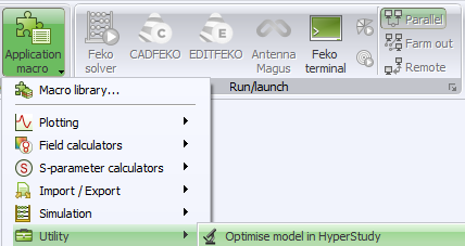
2. Click Application Macro under the Scripting group.
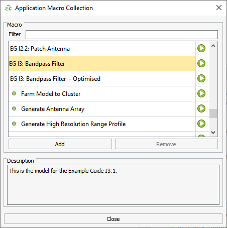
3. In the drop-down list, select Macro Library and run the EG I3: Bandpass Filter script.

   
   

   

   
   

4. Save the model with the name bandpassfilter.cfx and execute the solver.
5. Open the bandpassfilter.cfx model in POSTFEKO.
6. Create a Cartesian graph and add the S11 trace from the SParamOpt request.

   
   

   

   
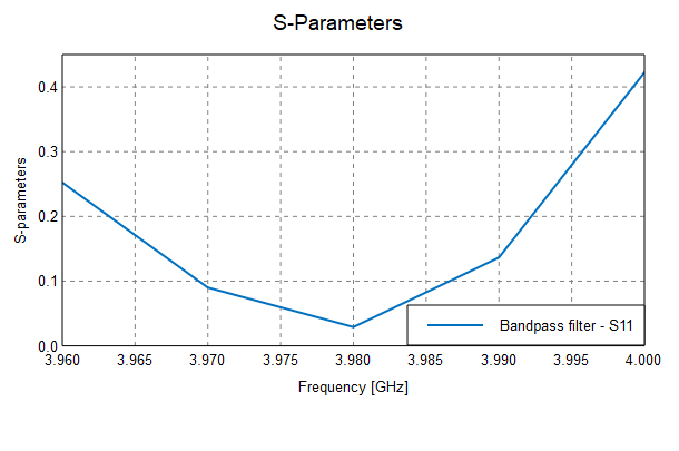
   Figure 1. The reflection coefficient (S11) of the bandpass filter before optimisation from 3.960 GHz to 4 GHz.

7. Save the bandpassfilter.pfs file in the same location as the bandpassfilter.cfx.
8. Click Application macro in the Scripting group.
   The scripts loaded in the Macro library is displayed.

   Figure 2. Example of the scripts available Application macro library.

   
   

   

   
   
9. Click Utility and select Optimise model in HyperStudy.
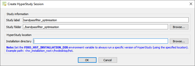
   The following Create HyperStudy Session dialog is shown.

   
   

   

   
   

10. In the Study label field, enter a value for the name of the study.
11. In the Study folder field, specify a value for the directory of the HyperStudy session.
12. In the Installation directory field, specify the directory where HyperStudy is installed.
13. [Optional] Set the FEKO_HST_INSTALLATION_DIR environment variable to use a specific version of HyperStudy.
14. Click OK to start to create a HyperStudy session.
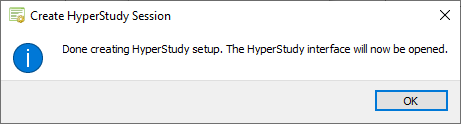
    The following Create HyperStudy Session dialog is shown.

    
    

    

    
    

    The extraction script bandpassfilter.cfx_extract.lua is created in the same directory as the bandpassfilter.pfs.

    Note: The trace on the Cartesian graph is extracted to the HyperStudy output file automatically. No additional scripting is required in the bandpassfilter.cfx_extract.lua file.

15. Click OK to launch HyperStudy.
16. Under Define models, verify the Solver Execution Script field is set to use the correct version.
    Note:

    • The script is accessible under Edit > Register Solver Script, which offers the possibility to register another solver or version.
    • The argument -np can be typed in Solver Input Arguments to specify the number of cores to use.
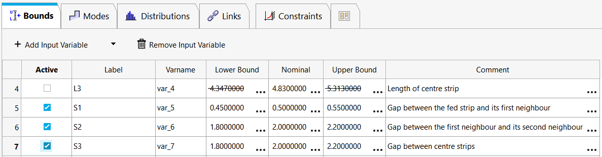
17. Under Define Input Variables, select which variables to include in the study. Only S1 – S3 should be activated and the default ranges used.
    An example of the selected variables is displayed.

    
    

    

    
    Figure 3. Example of the variable selection

18. Click Next.
19. Click Run Definition.

    
    

    

    
    Figure 4. Example selecting the Run Definition button.

    During the Write phase, the bandpassfilter.cfx_extract.lua file was copied to the run directory and executed after the Feko solver was run in the Extract phase. This generated an output file that HyperStudy can process easily.

    Note: The script bandpassfilter.cfx_extract.lua is different if a .pfs file was present before importing the variables and will automatically extract the visible traces on a Cartesian graph and polar graph.
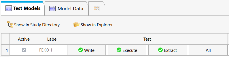
    See Figure 5 for the completed definition run for the Write, Execute and Extract phases for the initial test run done by HyperStudy.

    
    

    

    
    Figure 5. Example of the completed definition run.

20. Click Next.
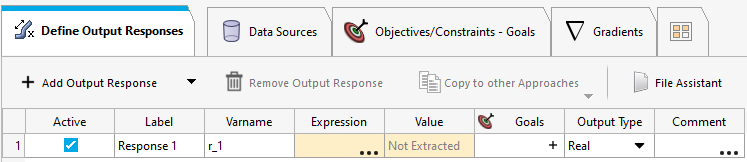
21. Select Add Output Response.
    An output response is added with the Expression field highlighted.

    
    

    

    
    

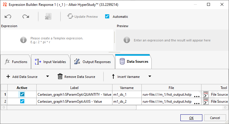
22. Select the Expression field.
    The Expression Builder:Response1(r1) dialog is shown.

    
    

    

    
    

    Note: The Data Sources m1_ds_1 and m1_ds2 is added from the POSTFEKO graph.

23. In the Expression field, enter max(m1_ds_1) and click OK.
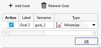
24. Under Goals click to add an optimisation goal.
    The following dialog is displayed.

    
    

    

    
    Figure 6. Example adding an optimisation goal.

25. Set the goal Type to Minimize and click OK.
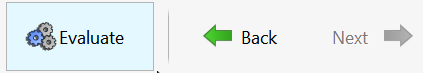
26. Click Evaluate to extract the value from the output file.

    
    

    

    
    Figure 7. Example selecting the Evaluate button.

    HyperStudy is now configured to understand which model to use, which variables are available for modification and how to process the output.
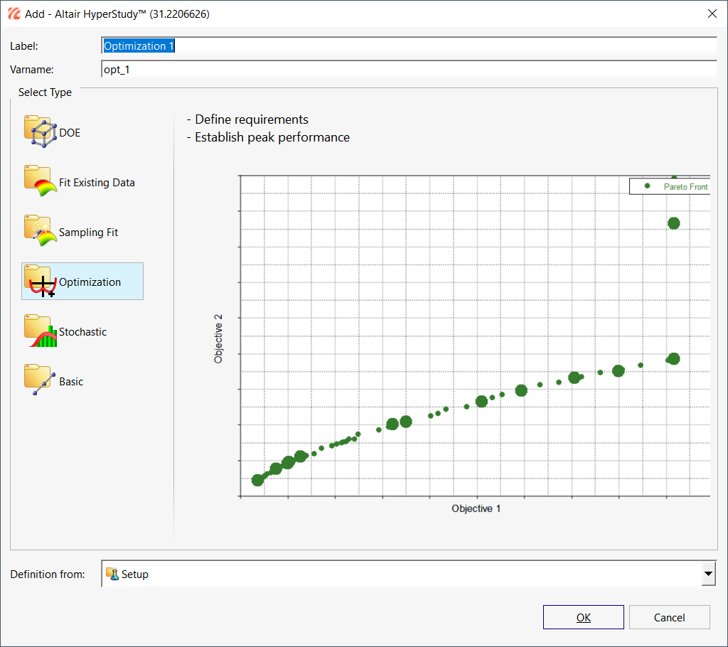
27. Right-click on the defined study in the Explorer tab and click Add.

    
    

    

    
    Figure 8. The Add dialog and selecting an optimisation approach.

28. Under Select Type, select Optimization and click OK.
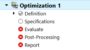
29. In the Definition from: drop-down list, select Setup and click OK
    The optimisation approach is created in the Explorer tab

    
    

    

    
    Figure 9. Example of the Optimisation 1 approach created.

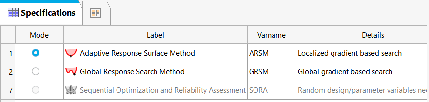
30. Click Optimization 1 > Specifications, and select the Adaptive Response Surface Method as the optimiser.

    
    

    

    
    Figure 10. Selecting the Adaptive Response Surface Method.

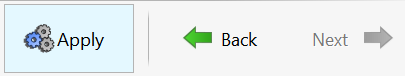
31. Click Apply and click Next.

    
    

    

    
    Figure 11. Example selecting the Apply button.

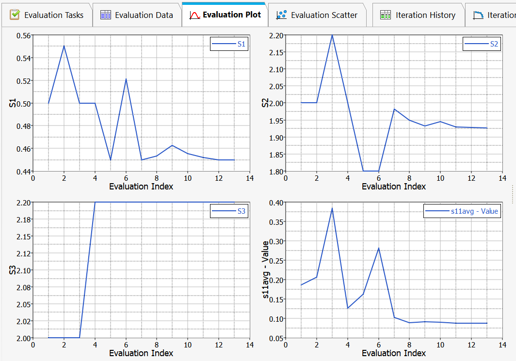
32. Click Evaluate Tasks.

    
    

    

    
    Figure 12. Example selecting the Evaluate Tasks button.

    Each of the input variables is altered randomly, and its effect on the response analysed.

    
    

    

    
    Figure 13. Typical progress data for an ARSM optimisation.

33. Click Iteration History tab and look for the row highlighted in green.
    The optimum values are as follows:

    • S1 = 0.4500000
    • S2 = 1.9254786
    • S3 = 2.2000000