Feko is a comprehensive electromagnetic solver with multiple solution methods that is used for electromagnetic field analyses
involving 3D objects of arbitrary shapes.
EDITFEKO is used to construct advanced models (both the geometry and solution requirements) using a high-level scripting language
which includes loops and conditional statements.
One of the key features in Feko is that it includes a broad set of unique and hybridised solution methods. Effective use of Feko features requires an understanding of the available methods.
Feko offers state-of-the-art optimisation engines based on generic algorithm (GA) and other methods, which can be used
to automatically optimise the design and determine the optimum solution.
Feko writes all the results to an ASCII output file .out as well as a binary output file .bof for usage by POSTFEKO. Use the .out file to obtain additional information about the solution.
The MRI application macro computes , , their ratio and the intrinsic signal-to-noise ratio (ISNR) for magnetic resonance imaging (MRI) investigations in POSTFEKO.
The radiation phase centre is a useful quantity to calculate, especially for reflector antennas. The phase centre calculation
is not available in Feko by default, but a stand-alone application macro is available that can be used to calculate the phase centre of a calculated far field.
The radiation phase centre of an antenna is the point from where the structure seems to radiate a spherical wave.
For an isotropic radiator, the phase centre would be the point where the isotropic radiator is located.
The phase centre can be calculated in multiple ways since no unique phase centre exists for a real antenna. It is
important to understand the difference between the methods to select the most appropriate calculation.
The methods (or functions) available include the two phase centre calculations, a method to translate a far field
to a new origin and a method to normalise (set zero phase reference) the phase of the far field.
The different methods provided by the phase centre application macro to calculate the phase centre of a simple horn antenna are utilised and the results are compared to illustrate their
differences.
This POSTFEKOapplication macro can be used to plot all the standard parameters that are available after a characteristic mode analysis simulation
was performed.
This application macro is used for calculating mean effective gain (MEG) and envelope correlation coefficient (ECC) for a MIMO antenna configuration.
The MEG ratio can also be plotted.
The Multiport post-processingapplication macro allows you to calculate results for changes in the port loading without rerunning the Solver. Results that are supported are far fields, near fields, currents and specific port parameters, for example,
the voltage, current and S-parameters of each port.
A Lua implementation of the transient Pennes bioheat equation using finite differences and explicit time stepping for calculating
thermal results in POSTFEKO.
The characteristic mode synthesis and design application macro is a post-processing application macro that can be used to calculate a weighted sum for the currents, near fields, and far fields requests for specific
characteristic modes of interest. The application macro uses a modified version of the modal weighting coefficient (MWC) to use the radiating phase when synthesising
the results with the macro.
CADFEKO and POSTFEKO have a powerful, fast, lightweight scripting language integrated into the application allowing you to create
models, get hold of simulation results and model configuration information as well as manipulation of data and automate
repetitive tasks.
The radiation phase centre is a useful quantity to calculate, especially for reflector antennas. The phase centre calculation
is not available in Feko by default, but a stand-alone application macro is available that can be used to calculate the phase centre of a calculated far field.
Use the first method in general and the second method when required.
The example illustrates that there is no single phase centre and that the best phase
centre calculation method depends on the requirements of the application. The phase
centre calculation at a single point (method 1) should be used in general, but the
second phase centre calculation method can increase the low phase variation area in
cases where this is required.
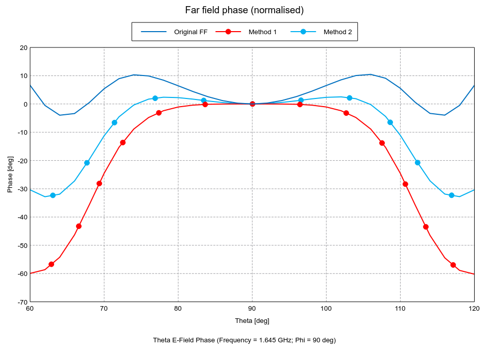
The graph (below) illustrates the phase variation in a single ϕ
cut. We can see that the original far field varied considerably and is not flat at
θ=90°. The first solution method is
perfectly flat at θ=90°, but quickly
deviates from zero when θ is more than 10° from the centre. The second solution method is not as flat as the
first, but the only starts deviating away from zero when θ is
more than 15° away from the centre.