EDEM Simulator

About the EDEM Simulator

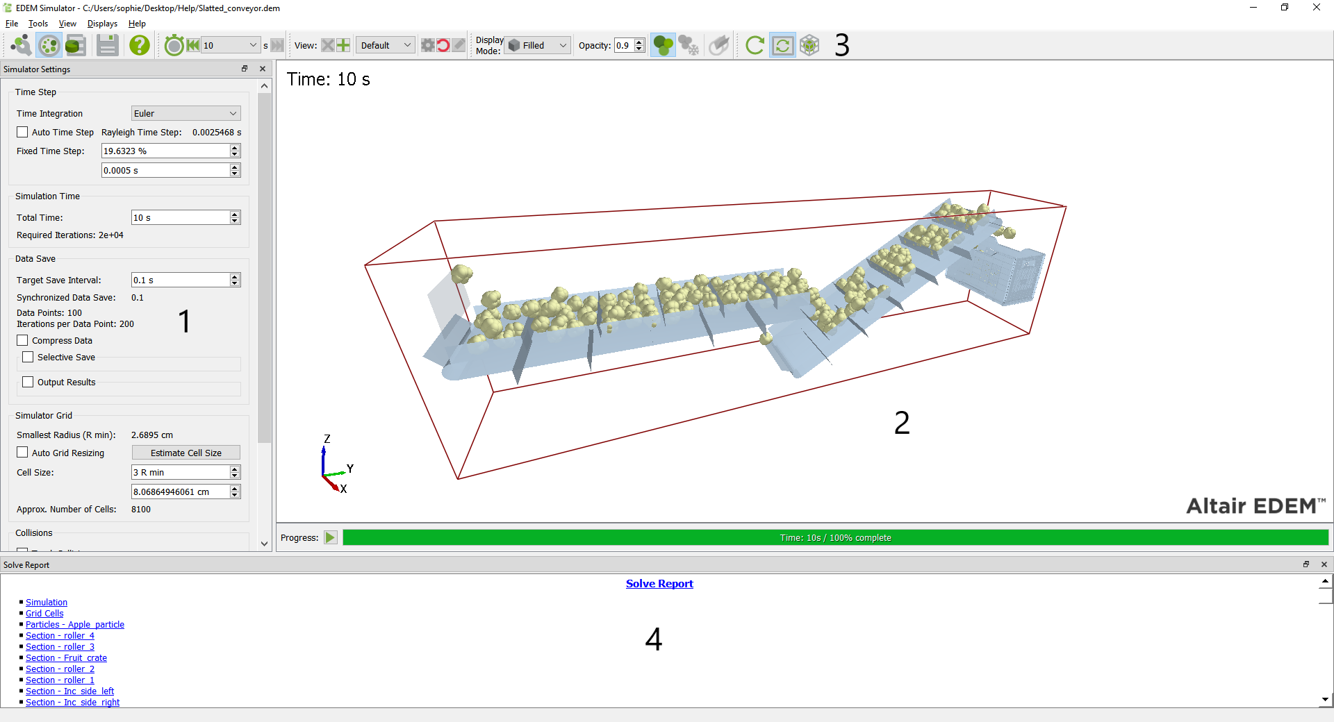
The Simulator is where you configure and control the EDEM simulation engine, and where you can observe the progress of your simulation.

 

1. Simulator Pane
2. Viewer
3. Toolbar and Menu Bar

4. Solve Report

Simulator Pane

The Simulator Pane is where the time step, simulation time, grid options and Simulator Engine are set for the CPU mode or the GPU parameters are set.

Viewer

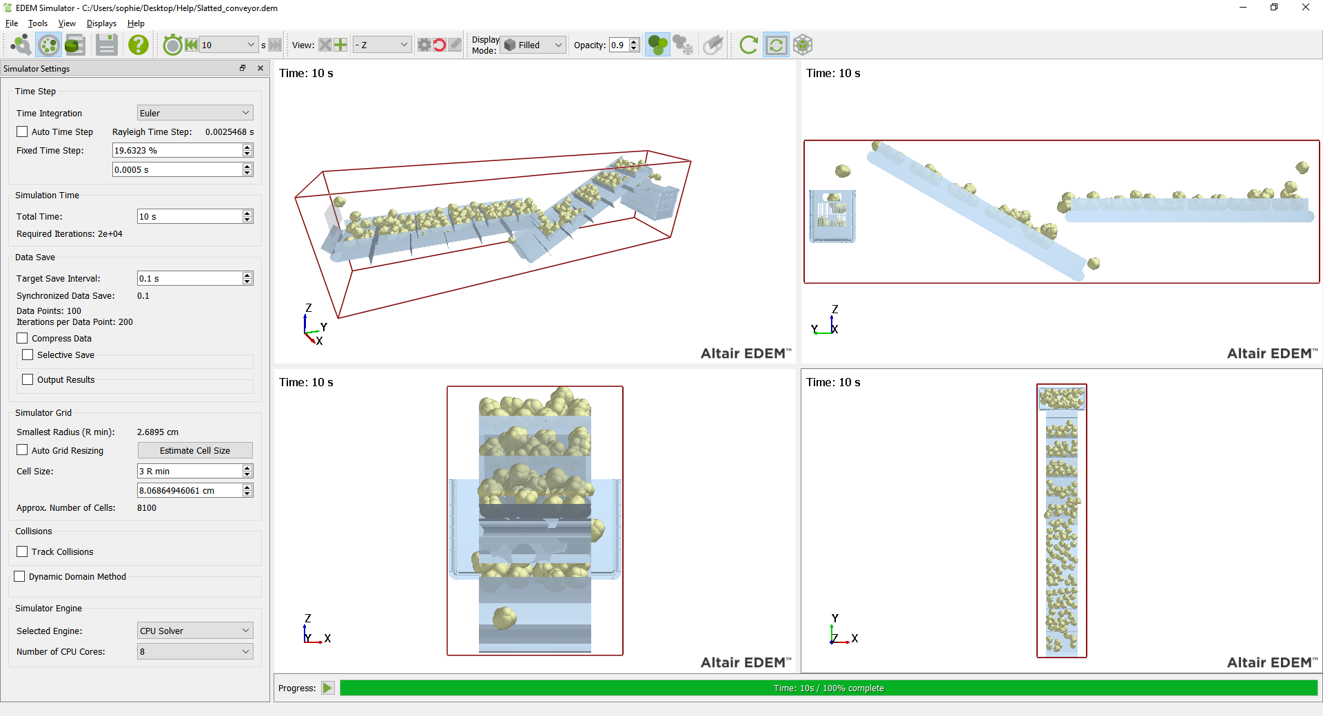
The Viewer displays 3D representations of your particles, geometry, and fields (if applicable). The rotation, position and zoom factor of the Viewer are controlled using the mouse. The user can set up more than one display splitting the screen in order to see the progress of the simulation from different points of view. The simulation start/stop button and simulation progress bar are just below the viewer.

Simulator Toolbar

Icon	Name	Description
	Creator	Switch to the Creator.
	Simulator	Switch to the Simulator.
	Analyst	Switch to the Analyst.
	Save	Save any changes made to Simulator settings.
	Help	View the online help.
	Change Time Step Back	Move to the first time step in the simulation.
	Change Time Step Forward	Move to the last time step in the simulation.
	Filled Display Mode	Click to display geometry filled.
	Mesh Display Mode	Click to display geometry as mesh.
	Points Display Mode	Click to display geometry as points.
	Display Particles	Show Particles in the Viewer.
	Display Frozen Particles	When checked and using the dynamic domain, any frozen particles will be colored black.
	Display Cylindrical Periodic Boundary Conditions	Displays cylindrical periodic boundary conditions.
	Show GPU Splitting Plane	Show/hide Multi-GPU split.  For the OpenCL solver this will display the user defined splitting plane.  For the CUDA solver this will color the particles depending on which card they are allocated to.
	Refresh Display	Update Viewer to show the 3D simulation at the Time Step when the button is pressed.
	Auto Update	Activate/Disable Auto Update.
	Simulator Grid	Show/Hide Simulator Grid.
	Coupling Server	Start Coupling Server.
	Coupling Server	Disable Coupling Server.

Viewer Controls

The Viewer Controls are used to determine how items are displayed in the Viewer.

• Current time. The current simulation time is displayed. Simulation can be stopped and any previous full time step viewed. Simulation can be restarted from any previous full time step.
• View. Controls to change, add, and configure camera views.
• Display mode. Configure the display of all the geometry in the Viewer. Choose between filled, mesh or points style display.
• Opacity. Set the opacity level of the geometry in the Viewer.

Simulator Menu Bar

File Menu

1. Save. Save any changes made to Simulator settings.
2. Import Config. Import a config (*.dfg) file.
3. Export Config. Export a config (*.dfg) file.
4. Creator. Select to switch to the Creator.
5. Simulator. Select to switch to the Simulator.
6. Analyst. Select to switch to the Analyst.
7. Quit. Quit EDEM.

Tools Menu

The Tools Menu in the Simulator is the same as for the Creator with the addition of the GPU Memory Calculator.

1. OpenCL GPU Memory Calculator
   The OpenCL GPU Memory Calculator is a tool to help estimate the memory required to run the current simulation. It also shows the memory available from the current GPU device so that the user can compare estimated memory usage with available memory, if the estimated memory usage is greater than the available memory the user can modify the settings below to optimize the GPU simulation memory usage.

   1. Total Available Memory Size: Shows the Memory available within the used GPU device, if a different GPU is used for display and processing the value available may not match the true amount available.

   2. Required Memory for Grid: Memory allocated to the domain grid.

   3. Required Memory for Particle: Memory allocated to particle data.

   4. Required Memory for Contact Cache: Memory allocated to the possibility of simultaneous contacts in 1 particle.

   5. Required Memory for Contact Storage: Memory allocated for contact data.

   6. Number of Particles: This value will define the amount of initial memory allocated for particles. The best option is to input the number if it is known. Otherwise, click on the green arrow to let EDEM estimate it from the factories already set in the Creator. While the default value is 100k, the minimum value can be set as 10k.

   7. Number of spheres (Multi-Sphere only): This value will define the amount of initial memory allocated for contact cache and contact storage. The best option is to input the number if it is known. Otherwise, click on the green arrow to let EDEM estimate it from the factories already set in the Creator. While the default value is 100k, the minimum value can be set as 10k.

   8. Number of Particle – Particle Contacts: The user can set it up if known. Otherwise, with the green arrow, EDEM will estimate an average of 3 Particle-Particle contacts per sphere. While the default value is 300k, the minimum value can be set as 10k.

   9. Number of Particle – Geometry Contacts: The user can set it up if known. Otherwise, with the green arrow, EDEM will estimate an average of 1 Particle-Geometry contact per sphere. While the default value is 100k, the minimum value can be set as 10k.

   10. Required Memory for Geometry: Memory allocated to the geometry mesh.

   11. Total Required Memory size: Total memory required by all the points above.

View Menu

1. Show Particles: Activate/deactivate to see the particles in the Viewer.

2. Parent-Child Lines: Shows lines to represent the Parent-Child relationships between geometries.

3. Themes: Show the EDEM interface with Legacy Theme (default) or Dark Theme.
4. Show Frozen Particles: When checked and using the dynamic domain, any frozen particles will be colored black.
5. Refresh Display: Update Viewer to show the 3D simulation at the Time Step when the button is pressed.
6. Auto Update: Activate/deactivate to apply Auto Update to the simulation in the Viewer.
7. Show Simulator Grid: Activate/deactivate to see the Simulator Grid.

Displays Menu

1. Show 1 Display

2. Show 2 Displays
3. Show 3 Displays
4. Show 4 Displays
5. Split Display Horizontally
6. Split Display Vertically

Help Menu

1. Help: The help menu brings up the relevant information regarding the EDEM interface.
2. About EDEM: The about box provides information about the current version of EDEM. The EDEM Version and Revision number are useful information to provide EDEM technical support when discussing support cases.
3. About Altair Simulations Products: The About Altair Simulation Products gives access to the Copyright notices, Altair website, License Agreements and Customer Support.

Solve Report

The Solve Report is an .html page that displays detailed information about your model. Right click anywhere within the Solve Report and choose Save to save the information in an .html file. The solve report details information from the last refresh point, this may not be the current simulation time. Right click on the solve report and choose 'refresh' to update the information shown to the current simulation time. There are six sections in the Simulator’s Solve Report:

Simulation

1. Status. Whether the simulation is processing or stopped.

2. Current time. Time into processing.
3. Time step. The time step used by the model as detailed in the Simulator.
4. Estimated total computation time. The estimated total time to complete the simulation.
5. Elapsed computation time. Time since the simulation started (excluding pauses).  Simulations which have been exported have the Elapsed time reset to 0 on export.

Grid Cells

1. Status. Either allocating grid cells or grid cells have been initialized.

2. Side length. The dimensions of grid cells as specified in the Simulator.
3. Created. The number of grid cells created.

Particles

1. Total number. The total number of particles in the model.

2. Total removed. The total number of particles removed from the model: for example, particles that move beyond the domain boundaries.
3. Minimum speed. The speed of the slowest particle in the model.
4. Maximum speed. The speed of the fastest particle in the model.

Geometry Section

1. Speed. The speed of the geometry section.

2. Number of particles in contact. The total number of particles in contact with the geometry section at the current time step.

Energy

1. System energy. The total energy in the model at the current time. It is the sum of the kinetic energy, potential energy and the energy in any contacts taking place. It should be equal to the total energy gained by creating particles plus the total energy gained by geometry movement minus the energy lost through contacts minus the energy lost by removing particles.

2. Kinetic & potential energy. The total kinetic and potential energy in the system.
3. Total lost by removing particles. Total energy lost by removing particles from the domain.
4. Total lost through contacts. Total energy lost by contacts between elements.
5. Total gained by creating particles. Total energy gained.
6. Total gained by external forces. Total energy gained from external forces.

Factory

1. Status. The current factory status.

2. A plot of the particles generated versus the factory settings.
3. Total particles created. Number of particles accepted and currently being generated.
4. Total particles regenerated. Number of particle creation attempts, if this number is significantly larger than the total particles created then it could be an indication that the simulation is running slowly due to excessive CPU effort going towards creating particles.
5. Total particles failed. Number of particles that could not be placed once the Max attempts to place particle is reached.
6. Total particles accepted. Number of particles accepted in the grid.
7. Creation rate/target creation rate. The particle or mass creation rate as specified in the Factories pane.
8. Mass created since rate change. Amount of mass created by the factory (when creation rate is set to target mass rate of particles).
9. Actual creation rate since rate change. The actual creation rate (as opposed to the target creation rate) when creation rate is set to target mass rate of particles.

Simulator Settings

Time Step

The time step is the amount of time between iterations (calculations) in the Simulator. The time step is either fixed and remains constant throughout the simulation or the Auto Time Step option can be chosen.

The value is displayed as both the actual time step (in seconds) and as a percentage of the Rayleigh time step. The Rayleigh time step is the time taken for a shear wave to propagate through a solid particle. When using a simulation with a range of particle sizes, the Rayleigh time step is calculated based on the smallest particle size.  This means during a single time step disturbances cannot propagate further than the immediate neighbors. Based on this the resultant forces on a particle are determined exclusively by its interactions with particles with which it is in contact. It is also assumed that all energy is transferred via Rayleigh waves.  When using a normal distribution the time step is set based on the lower capped value, if no capping is used the time step is set based on the particle which has size ‘mean – 3 * standard deviation’.

The smaller the time step, the more data points are produced. A large number of data points produce results with a very fine level of detail; however, the simulation time will be longer due to the increased number of calculations required.

Sphero-Cylinder Time step

The Rayleigh time step for Sphero-Cylinder particles is currently calculated in the same way as for multisphere particles using the Sphero-Cylinder radius. It does not take into account the length of the Sphero-Cylinders and users should be aware that a smaller fraction of the Rayleigh time step may be needed in cases with large aspect ratio particles.

Polyhedral Time step

The Rayleigh time step is the only type of time step automatically calculated for polyhedral particles. To calculate the Rayleigh time step for polyhedral particles, the effective radius of the smallest particle, Reffective is used.

Choosing a Time Step

Typically a time step is chosen as a percentage of the Rayleigh time step value. The normal range is 10%-40% of the Rayleigh time step, the higher the particle energy in the simulation (higher forces, faster collisions) the lower the time step value.  20% of the Rayleigh time step is the default value recommended.

The Rayleigh time step is based on Particle elements only, if using models with additional elements (such as bonds), alternative time step methods should be considered.

If the time step is too small, the simulation will take a long time to run. If the time step is too large, particles can behave erratically. For example, the figure below shows two particles moving towards each other. At time step 1 they are some distance apart. The particles are moving towards each other at some speed, and when their positions are recalculated at time step 2 they are apparently over-lapping. The particle forces and energies are recalculated at this point; however, these values are very large due to the apparent overlap; this supplies each particle with a very large and incorrect velocity, and they move off erratically at time step 3. Subsequently, these particles can come into contact with other elements in the system, often causing an 'explosion' of incorrectly moving elements.

 

1. Auto Time Step: If this box is ticked EDEM will automatically adjust the Rayleigh time step to the smallest radius that is currently in the simulation rather than the smallest radius to be created. It uses 20% for this particle size. For example, a simulation that has 10 mm particles  from t=0s and 3 mm particles from t=3s will use 20% of the Rayleigh Time Step obtained with 10mm until time 3s, when it would be updated to the Time Step value obtained with 3mm.

2. Time Integration: Select the desired time integration scheme between Euler, Position Verlet and Velocity Verlet.

   1. Euler: Euler is a first-order time integration method and is used as the default time integration method for EDEM.

   2. Position Verlet, Velocity Verlet: Position Verlet and Velocity Verlet are integration methods of second order. Velocities and positions are calculated for time steps which are t/2 apart. The Verlet methods come at a slight additional computational cost (up to 10%); however, the methods come with increased computational accuracy. Note only compatible with MultiSpheres.

Simulation Time

The simulation time is the amount of real time your simulation represents.

1. Total Time: The total actual length of the simulation in seconds or minutes.
2. Required Iterations: Indicates the number of iterations required to complete a simulation of a defined time using the defined time step. For example, 5e+05 iterations are required to produce one second of simulation with a time step of 2e-06.

Data Save

1. Target Save Interval: How often data should be written out to a file. This determines the number of data points (the points at which data is collected from the simulation for analysis).
2. Synchronized Data Save: The actual time that data will be saved. This is usually the same as the target save interval,  but may differ depending on the time step time.
3. Data Points: The number of data points as determined by the target save interval, It is calculated as the total run time divided by the target save interval.
4. Iterations per Data Point: The number of simulator iterations for each data point.

Selective Saves

When simulating, EDEM saves particle, geometry, and interaction data for post-processing and analysis. Often you may only be interested in a subset of this data: EDEM’s selective save feature lets you select which attributes are saved and how often by defining partial saves. Using selective save can greatly reduce simulation data file sizes as well as enabling you to run even larger simulations.

Selective save works by combining full saves (where all data is written out) and partial saves (where only selected data is written out) to create smaller data sets. For example, assume you have a simulation with a total time of 10 seconds that writes-out every 1 second. By default, this creates a full save of all simulation data every second:

0s	1s	2s	3s	4s	5s	6s	7s	8s	9s
Full	Full	Full	Full	Full	Full	Full	Full	Full	Full

 

Setting the Full Data Save Every option to e.g. 3 intervals results in a full save only every 3 seconds (the first write-out is always a full save):

0s	1s	2s	3s	4s	5s	6s	7s	8s	9s
Full	Partial	Partial	Full	Partial	Partial	Full	Partial	Partial	Full

 

To enable selective save:

1. Tick the Selective Save checkbox.

2. Enter a value into Full Data Save Every to set the frequency of full data saves. For example, set this to create a full save every 5 intervals.

3. Click the Configure Save button. The Data Save Configuration window is displayed.

4. Select which particle, geometry, and interaction attribute data to save in a partial save. Use the appropriate checkbox to include an attribute in the save. Any other required attributes will also be enabled. Untick a data group to exclude related attributes.

The Data Save Configuration window also displays an estimate of the per-particle or per-triangle reduction in data size for each time step.

Note that if you stop the simulation early then switch to the analyst, the current time step will be a full save irrespective of the full save interval.

Particle Data

Data Group	Attribute Data
Base Particle Data	ID
	Position
	Orientation
	Number of Particles
	Volume
	Voidage
	Mass
	Moment of Inertia
	Potential Energy
Velocity	Velocity
	Kinetic Energy
Angular Velocity	Angular Velocity
	Rotational Kinetic Energy
	Total Energy
Force and Torque	Compressive Force
	Total Force
	Torque
Custom Properties	Custom Property

Geometry Data

Data Group	Attribute Data
Base Geometry Data	ID
	Position
	Surface Normal
	Node
	Number of Geometry Elements
	Velocity
	Angular Velocity
Force and Torque	Compressive Force
	Total Force
	Torque
Custom Properties	Custom Property

Interaction Data

Data Group	Attribute Data
Contacts (Particle-Particle)	All particle-particle contact attribute data.
Contacts (Particle-Geometry)	All particle-geometry contact attribute data.
Collisions (Particle-Particle)	All particle-particle collision attribute data.
Collisions (Particle- Geometry)	All particle-geometry collision attribute data.
Bonds	All bond element attribute data.
Custom Properties	All interaction-based custom property data.

Output Results

While simulating, EDEM can export simulation results. This is useful to assess the behavior of your simulation during processing without the need for stopping and post-processing in the EDEM Analyst.

First setup a config query in the EDEM Analyst > File > Export Results data. Multiple export data Configs can be setup however only one can be used to output results in the Simulator.

When in the EDEM Simulator enable the Output Results tick and choose one of the available export data Configs.  The data exported is governed by the Configuration ID chosen.

The exported data corresponds directly to the query defined in the Analyst, including name and location of the CSV file. See Analyst > Exporting Data for more information.

Simulator Grid (OpenCL and CPU Engine only)

 

Collisions (CPU only)

Storing Collision Data

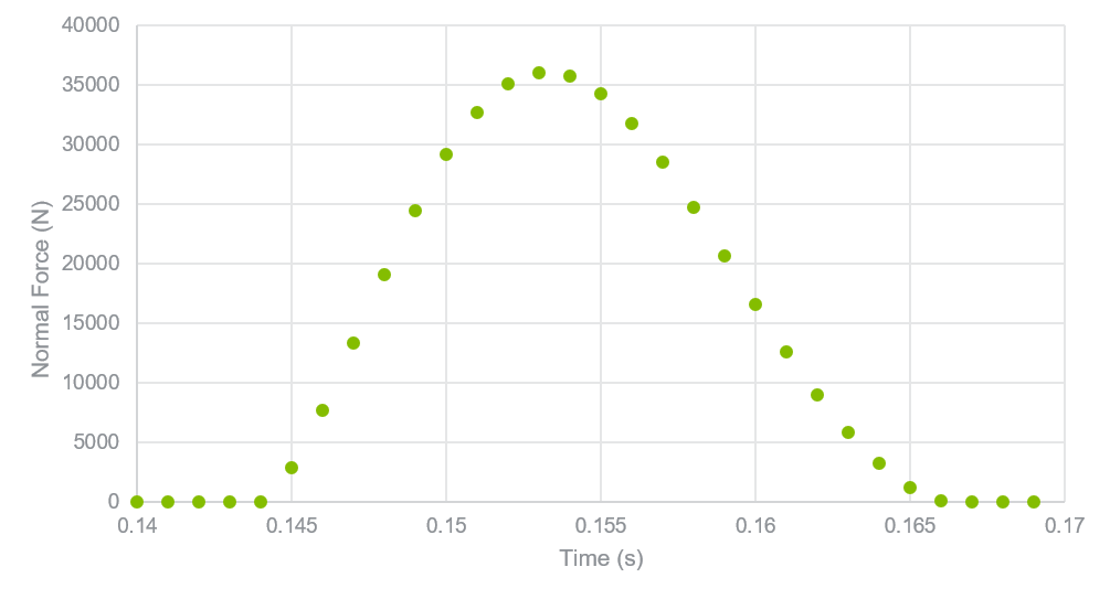
Example force-time graph for a single particle-geometry collision where each point is a contact

 

During a simulation data can be recorded about both contacts and collisions.

 

1. Contacts are the impacts occurring between elements at data write-out points. In other words, the contact is in progress when the write-out takes place. The contact has an associated force, position and so on - these are discrete values. If two elements stay in contact with each other for some time e.g. over 4 write-out points, four contacts will be stored and each of these may have a different force, position and so on.

 

1. Collisions are complete impacts.  When two elements collide it will register as one collision, regardless of how long the elements stay in contact for.  Data is collected for the duration of the collision e.g.  total energy loss, min/max/average normal force data and so on. Collisions may occur in-between write-outs and never register as contacts.

 

EDEM records all contact data as standard. To record collision data, enable Track Collisions. Storing collision data will significantly increase memory usage and reduce the speed of the simulation. Collision data is stored in memory until it is written out at the rate specified in the Simulator. If a large number of collisions are occurring and the write out frequency is too low, the amount of data being stored in memory will become very large and use up all memory resources. To minimize this, be sure data is written out frequently.

As of EDEM 2020.1 the forces reported by EDEM for collisions are undamped.

 

Energy Loss

Energy loss in a collision between two elements (particle-particle or particle-geometry) lasting n contacts over time is calculated by:

 

 

Where…

 

F	=	Contact force [N]
Vi	=	Relative velocity after contact [ms-1]
Vi-1	=	Relative velocity before contact [ms-1]
dt	=	Time step [s]

Simulator Engine

A simulation can run in CPU mode or in GPU mode. GPU mode requires supported GPU hardware. There are two GPU engines, the CUDA engine and the OpenCL engine.  The CUDA engine will run Polyhedral, Sphero-Cylinder and Multi-Sphere simulations and requires a suitable Nvidia graphics card. The OpenCL engine will run Multi-Sphere simulations and will run on any graphics card which support OpenCL.

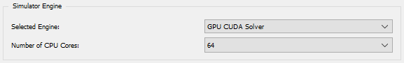
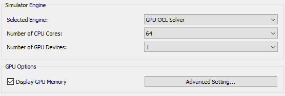
Selected Engine

The user can choose between CPU, OpenCL or CUDA Engine. If the GPU option is not available please check GPU compatibility:

 

 

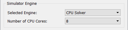
CPU solver shown above. The user can select the number of CPU cores, the number available depends on the CPU hardware available

 

 

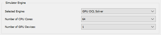
GPU solvers chosen from the Selected Engine above.The number of GPU devices can be set. In addition, the user selects the number of CPU Cores, as the processing is handled by the GPU card up to 4 CPU’s are recommended as the optimal value.

Check CUDA GPU Compatibility

GPU CUDA engine requires your GPU device to support Nvidia CUDA 11.2 or above. To check hardware compatibility with the GPU go to Tools > Options > Simulator Engine and select the GPU’s from the list and then choose Start test. As shown below EDEM will report if the test and GPU setup is successful. If multiple GPU devices are found a test should be run on each GPU device required to run EDEM.

 

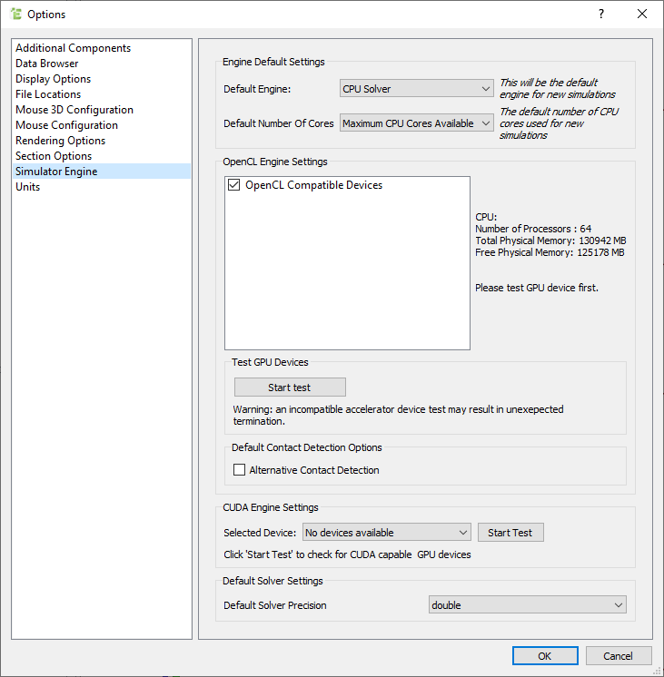
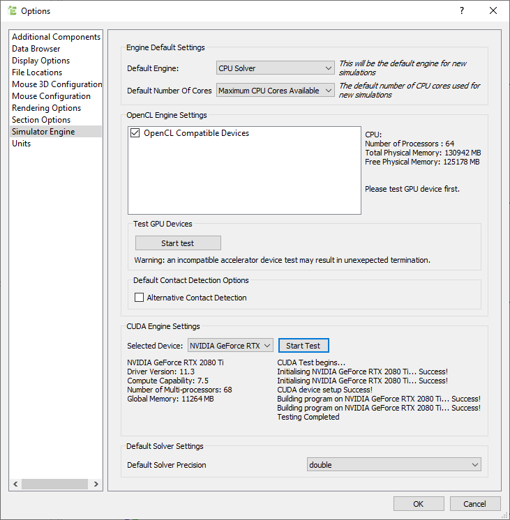
The test is a standard hardware test for Nvidia CUDA GPU. If the test fails, please make sure your Graphics Card drivers are up to date and try again or contact support with details of the GPU device used.

Only once the test has been run successfully will the GPU option be accessible from the Selected Engine dropdown menu.

Simulator Engine – GPU CUDA Solver

When the CUDA GPU Solver engine is selected, you are presented with the following options and information:

 

 

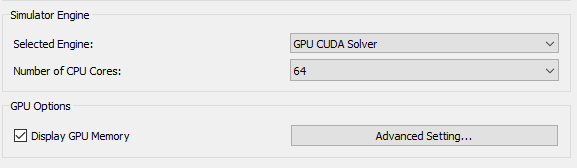
1. Number of CPU Cores – The CUDA GPU engine works with both CPU and GPU. The recommended number of CPU cores when running CUDA GPU is 4 as this provides a good balance of speed vs. CPU use.

2. Total available memory size:  This value shows the value in Megabytes that the percentage above represents for the selected GPU device.

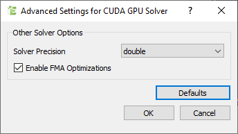
GPU CUDA Advanced Settings

The advanced options for the CUDA GPU solver allow users to modify the precision used for the simulation and disable FMA optimizations.

 

 

 

EDEM allocates a set number of bytes of memory to store simulation information, such as particle position or velocity. The larger the number of bytes it allocates the greater the precision EDEM can work with. By default, EDEM simulations use 8byte or "Double" precision storage. This means that information is stored at a very high precision. In many applications this level of precision is excessive and has a negligible benefit to the accuracy of simulations. High precision also slows down simulations due to the extra computational expense required to perform operations and slower memory storage/management.

Therefore, there are significant speed benefits to using the lower precision "Single" data type which only uses 4 bytes. It is possible that only using Single precision data may lead to noticeable differences in simulation results, compared to Double precision.  Rather than solely using either Single or Double precision a combined, Hybrid, approach can be taken. This is achieved by storing key simulation parameters (such as particle position) in double precision and using Single precision for the remaining properties. The result of this method produces simulations running nearly as fast as solely using single precision, whilst maintaining most of the accuracy of double precision. In order to maintain most of the accuracy of Double precision, storage of key simulation properties is, whilst gaining the computational speed a mixture of these data types can be used in a Hybrid method.

The following precision methods are available in EDEM:

 

Double:

1. Standard data type for EDEM
2. Highest precision
3. Slowest simulation speed

Single:

1. Lowest precision
2. Computational speeds up to 2.5x faster than double

Hybrid:

1. Strategic usage of Double and Single precision
2. Computational speeds up to 2.5x faster than double

 

Disabling FMA in CUDA

There is an optimization applied by the CUDA compiler known as 'fused-multiply-add' which combines addition and multiplication into a single instruction. More information is available here: https://docs.nvidia.com/cuda/floating-point/index.html#fused-multiply-add-fma.This will give improved performance, however there are some cases where it can cause the simulation results to change by a small amount. Therefore it can be helpful to disable this option when developing new code and trying to compare results between versions. This optimization can be disabled by passing the command line option --nofma=1 or by disabling it in the "Advanced Setting" dialog in the simulator options. Please note that this is a technical option and most users should leave it enabled which is the default.

 

Check OpenCL GPU Compatibility

EDEM GPU OpenCL engine requires your GPU device to support OpenCL 1.2 or above. To check hardware compatibility with the GPU go to Tools > Options > Simulator Engine>OpenCL and select the GPU’s from the list and then choose Start test. As shown below EDEM will report if the test and GPU setup is successful. If multiple GPU devices are found a test should be run on each GPU device required to run EDEM.

 

 

 

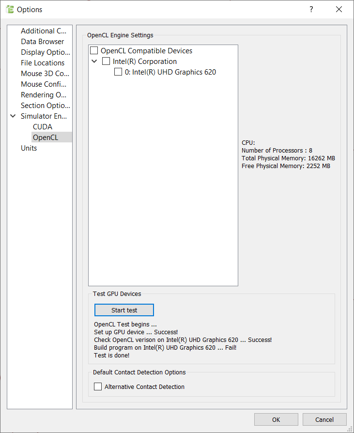
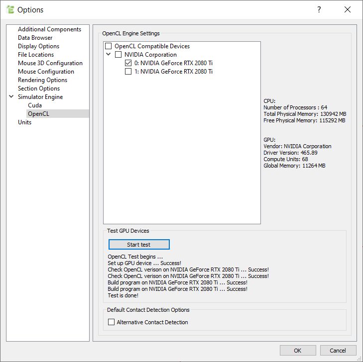
The test is a standard hardware test for GPU. If the test fails, please make sure your Graphics Card drivers are up to date and try again or contact support with details of the GPU device used.

Only once the test has been run successfully will the GPU option be accessible from the Selected Engine dropdown menu.

Simulator Engine – GPU OpenCL Solver

When the OpenCL GPU Solver engine is selected, you are presented with the following options and information:

 

 

1. Number of CPU Cores – The GPU engine works with both CPU and GPU. The recommended number of CPU cores when running GPU is 4 as this provides a good balance of speed vs. CPU use. If using the GPU with the EDEM API then the API models run on CPU when the contact detection runs on the GPU. As such, depending on the complexity and definition of the API model more than 4 CPUs may provide the optimal speed.

2. Number of GPU Devices – This displays the Number of GPU Devices available on the installed GPU hardware, this is not a value that can be modified by the user. The definition of Compute Unit differs depending on the GPU manufacturer. A compute unit is a Stream Multiprocessor for an NVidia GPU or a SIMD engine in an AMD GPU. For Nvidia each stream multiprocessor has a certain number of processing elements or what Nvidia calls ‘CUDA Cores’. Typically the more processing elements the faster the GPU card.

3. Available memory percentage: Indicates the maximum % of the computer’s graphic memory that EDEM is going to use. The default value is set to 75% in order to allow some memory for other non-EDEM related processes.

4. Total available memory size:  This value shows the value in Megabytes that the percentage above represents for the selected GPU device.

GPU OpenCL– Advanced Settings

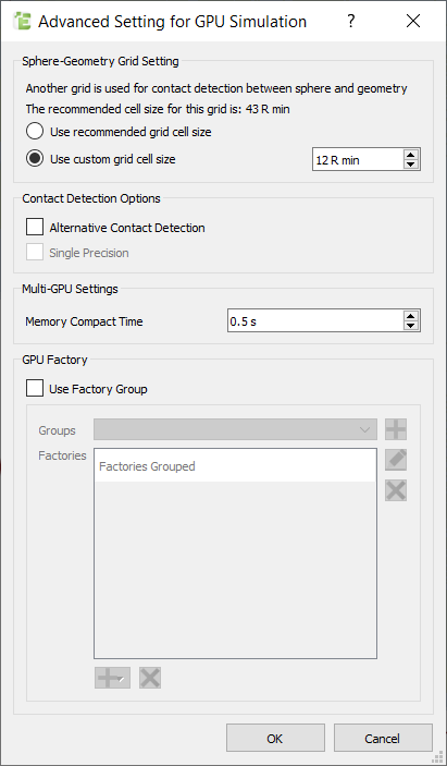
When selecting the GPU solver engine the GPU Advanced settings are available:

 

1. Sphere-Geometry Grid Settings – The user can set the Sphere-Geometry (Particle-Geometry) grid settings to be a different value to the Sphere-Sphere grid.  The default recommended value targets the fastest simulation speed for GPU however the user can also set their own custom value for this.

2. Alternative Contact Detection - The alternative contact detection method is a hybrid contact detection option which switches between two algorithms depending on simulation settings.  The algorithms primarily offer benefits when working with a large particle size distribution or with a domain consisting of small amounts of empty space. In these situations memory usage should be reduced resulting in an ability to run larger simulations in comparison to the standard contact detection method.

3. NB. This feature is available to use but it is advisable for the user to test if gains are achieved before activating for mainstream work.

4. Multi-GPU Settings– “Memory Compact Time” defines an interval at which Multi-GPU simulations will do a memory compact - reducing the physical GPU memory used while running Multi-GPU simulations. This is achieved by removing unused blocks of memory generated when particles pass from one GPU domain to another. This same process happens during regular save internals so “Memory Compact Time” will only have a significant impact when saving infrequently (i.e. when Save Interval > Memory Compact Time). Default value is 0.5 s and it is not advised to use very small values since this will impact simulation performance.

5. GPU Factory - If ‘Use Factory Group’ is selected then this allows the user to group particle factories together. All the particles in a simulation are created and tracked within factory domains by the CPU. The CPU will stop processing these particles and hand them over to the GPU once they leave the factory domain. If they re-enter or cross any factory domain afterwards, the CPU will not acknowledge them. Any particles re-entering the factory will likely lead to a particle explosion in the factory domain.
   
   To avoid this unexpected behavior, if several factories are close to each other and the particles might pass through each other’s factory domain, the user can enable “Use Factory Group”. This feature allows the user to group several factories together in order to make EDEM deal with them as one factory domain through the CPU.
   
   The larger the number of particles inside the factory domain (one factory or one group of factories), the higher the CPU usage and the lower the GPU usage involved. In extreme cases, where the factory covers the whole domain, all particles would be processed by CPU.
   
   At the same time, EDEM will detect when a factory stops generating particles. Hence, the corresponding factory domain would become invalid and all the particle information within it would be handed over from CPU to GPU to proceed with the calculations.

   1. Use Factory Group checkbox: Enable/Disable the use of factory groups in the GPU simulation.

   2. Groups: The dropdown list shows all the factory groups already defined. Add/delete a new group by clicking on the green/red crosses next to the selected group. The user can also rename a Factory Group.

   3. Factories: The box shows the Grouped Factories within the highlighted Group in the “Groups” dropdown list. Factories can be added and removed with the green/red cross below the Factories box. Any factory defined in the creator that has not been used in any other Factory Group will be selectable for a new grouping.

Number of Cores

This enables the number of processor cores used in the simulation to be specified via the Number of Cores dropdown. When you start a simulation, EDEM checks out the requested number of units from the license system (if available).

 

If your computer has hyper-threading enabled, EDEM will include these in the number of processors but these will not provide the same performance improvement as real cores.

Dynamic Domain

When a geometry object is defined as Dynamic Domain, all material inside the object will be active and any stationary material outside the object will be excluded from any calculations, which improves simulation speed.  A particle excluded from any calculation is called a frozen particle. If a frozen particle re-enters the dynamic domain then it is automatically included in the calculations again.

To use this feature, a geometry section must first be defined as a Dynamic Domain in the Creator. To do this, right click on the Geometries section, select Add Geometry and choose Box. Rename the new geometry and set the Type to Dynamic Domain. Please note, since the Bulk Material will not physically interact with the Dynamic Domain object, there is no option to assign material when dynamic domain has been selected.

Next, set the dimensions of the Dynamic Domain object suitable for the simulation, any material inside the domain will be active and any outside may become frozen.

In the Simulator there are three main parameters for Dynamic Domain.

Check Interval

If the particle does not move in this time interval and it is outside the Dynamic Domain then the particle is flagged to be frozen.

Number of Checks

This determines the number of times EDEM will perform the check to see if a particle is to be frozen.

Displacement of Particles as a Percentage of the Radius

This is the condition that determines if the particle is stationary or moving. If the displacement of the particle within the Check Interval is greater than this value then the particle is considered to be moving, otherwise it is stationary and can be removed from the force and contact detection calculations.

 

Dynamic Domain is based on the method outlined in Mio et al., 2009.

Dynamic Domain – Known Issues

1. Dynamic domain is not compatible with multi GPU.

2. Frozen particles do not apply forces on geometry sections.
3. Frozen particles are excluded from Contact Detection, forces and velocities are not computed.

Starting and Stopping a Simulation

The start/stop button is used to start and stop the simulation:

 

 

 

The current simulation time is shown in the Viewer Controls pane. All previous time steps are also listed. You can start and stop the simulation from any time step (current or previous) using the start/stop button. Simulations can also be stopped using the keyboard shortcut Ctrl + Shift + K.

 

Reducing Simulation Time

The following can help to reduce processing time.

 

1. Adjust the Simulator grid size.
2. Check the Factory is working effectively.
3. Save less data to the disk.
4. Turn off the display auto-update option (minor).
5. Activate the Dynamic Domain to freeze non-moving particles.
6. Turn off data compression

Simulation Parameters

The time taken by the Simulator to perform a single iteration, t_iteration, is affected quite significantly by the simulation parameters. An obvious parameter is the number of elements (particle surfaces and geometry elements) to be simulated. Consider if everything currently within the simulation is necessary to achieve a good result.

Extra parameters such as geometry dynamics and contact models can add to the computational overhead, especially complex models such as Hertz Mindlin with Bonding.

Grid Size (CPU and OpenCL only)

The fewer particles per grid cell, the more efficient the simulator. If there is no more than one particle in each grid cell then no contact detection needs to take place so the simulation will progress faster. The idealized length of a grid cell is typically in the range of 2-6-R_min where R_min is the minimum particle radius in the simulation, the lower the R_min value the greater the amount of Memory (RAM) used.

More grid cells require more system RAM so with large simulations the user needs to be aware of the total amount of RAM which EDEM is consuming and ensure this is below the RAM available. This should be the physical RAM available, not paged, as swapping to the hard disk is slow by comparison. Also be aware that memory usage will increase if there are still further particles to be introduced. The size of the Domain will also affect the number of grid cells required so consider if it can be reduced.

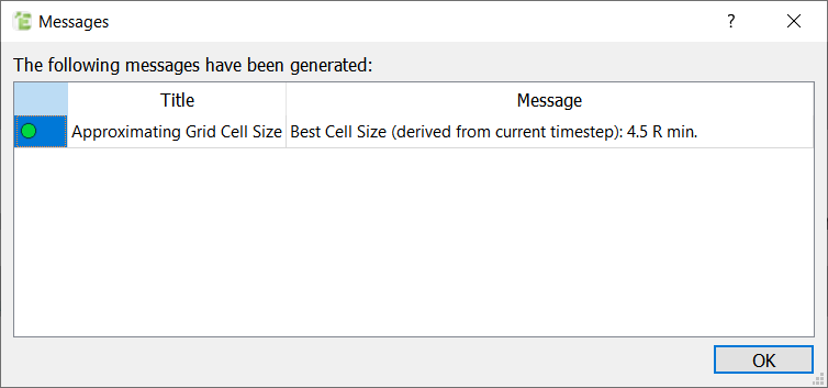
Estimate Cell Size

The estimate cell size is a heuristic algorithm which, based on the current simulation time step, will estimate the best cell size. Choosing this option will launch the approximation program and return an estimated best value for simulation performance:

 

Auto Grid Resizing

When Auto Grid Resizing is enabled, EDEM will assess different grid size settings and estimate the best value to continue the simulation with. The check will be performed at the same frequency at which the Data Write Out occurs and the calculated value will automatically be applied before continuing with the simulation. The algorithm will test a range of grid cell sizes between 3 Rmin and 15 Rmin and assess how many contacts will be generated at each setting. It will then use these results to find the setting where the minimum amount of contacts will occur.

Particle Factories

Particle Factories use contact detection to place each particle in a free region of space and any failed attempt will need to be repeated (up to max number of attempts). A Factory attempting to place particles in a region with a high particle volume fraction will significantly affect the simulation speed as the factory will find it more difficult to place each particle. If the particle volume fraction is above 25% (or lower for large size distributions), consider making the factory zone bigger or use a different approach to introduce particles. Use the Solve report to find out the number of particles which are ‘regenerated’ by the factory, ideally this should always be less than the number of particles created.

Save Less Data

Writing data to a hard disk is much slower than writing to memory so make sure only required data is saved. Increase the write-out period if possible or use Selective Save to only store the data which is of interest.

Auto Update Option

When the Auto Update option is selected (from the Viewer controls pane in the Simulator), the Viewer is regularly updated so the user can observe progress. Reduce the computation required by ensuring Auto Update is off (or EDEM is minimized) when observation of the simulation is not required.

The default value for auto-update is on.

Turn off data compression

When the data compression option is turned on the amount of hard drive space taken up by the simulation will decrease, however the compression of the data increases the simulation time.  Turning the compression off will speed up the simulation but will also increase the hard drive space used by the simulation.

This is set to be off by default.

Hardware and Drivers

t_iteration is affected by the amount of memory available to the software. Of equal importance is the type of memory, the processor(s) and the communication between the two. A faster processor is capable of carrying out more calculations per second and adding extra processors allows for the total computational load to be divided. The EDEM team has good links with hardware vendors and tests are continuously under way on possible speed improvements through hardware.

In addition to the hardware, maintaining up-to-date drivers can also help.

 

	(c) 2022 Altair Engineering Inc. All Rights Reserved. Intellectual Property Rights Notice | Technical Support