Brushless DC (BLDC/PMSM) motor tutorial: target tracking system

Model:  Target Tracking

Location: Examples > eMotors > eMotor Tutorials

This example simulates a servo-controlled positioning system that maintains focal plane line of sight coincident with target angle. The permanent magnet synchronous motor model is selected as an actuator to provide fast response.

Motor Specifications

Automatically acquiring and maintaining the line of sight of a video camera or focal plane sensor is often required in various aerospace, defense, and security system applications. One way to mechanize such a system is to reflect the field of view through two independently-controlled mirrors that each rotate in axes orthogonal to one another. The object of the control system is to acquire the target, and by controlling rotation of each mirror, move the line of sight coincident with the target angle. This places the virtual image of the target in the center of the focal plane. Once the image of the target is acquired on the focal plane, an error in azimuth and elevation can be determined by a variety of image processing techniques, such as contrasting, differencing, and area parameter calculations.

For this simulation, such a mechanism is assumed, with a pipeline image processor providing direct angular azimuth and elevation measurements. The following design decisions are also assumed:

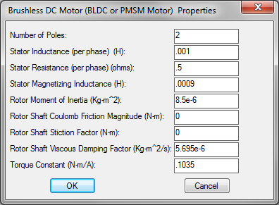
Motor type: Permanent magnet DC synchronous motor with Hall sensors for commutation sensing and control.

For the simulation, the Brushless DC (BLDC/PMSM) Motor block is used, along with the Hall Sensor block for commutation.

Power Electronics: Brushless PWM servo amplifier with speed and current Control. The base frequency of the PWM is 9000 Hz.

For the simulation, the PWM Brushless Servo Amplifier block is used

Precision current sense resistors produce voltage that is fed into a processor. An encoder provides motor shaft position and velocity. Encoder angle measurement and phase current measurements are used to obtain direct and quadrature current estimates through Clarke and Park transforms. Current and speed loops are used to set stiff inner loop performance.

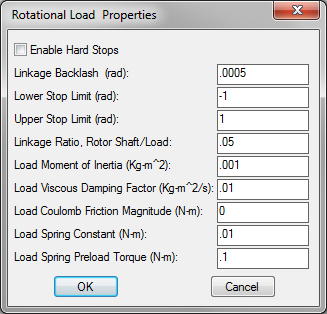
Mechanical Load: Precision λ/4 flat oval mirrors mounted on a gear reducer shaft with rotation center coincident with reflecting surface represent the main load moment of inertia. A torsional spring with preload tension is used to help minimize backlash hysteresis. An optical encoder is provided with 16000 lines to measure mirror angle. PI compensation is used for controlling line of sight. Load parameters are:

Gear reduction                       20:1

Backlash                                     0.0005 radians

Load moment of inertia      0.001 kg – m2

Load viscous damping        0.01 kg – m2/s

Load spring constant          0.01 N-m/rad

Load spring preload             0.1 N-m

Pipeline Image Processor: Provides 60 Hz frame rate acquisition of target from focal plane array. Pixel resolution is sufficiently higher than expected control requirement of less than ± 3 degrees between target angle and line of sight in both axes. Hierarchical classification and size discrimination of blobs with subsequent calculation of the target centroid determine target position.

Simulation development

From the eMotor toolbox, place the following blocks in your diagram:

•      PID Controller (Digital)

•      Hall Sensor

•      PWM Brushless Servo Amplifier

•      Rotary Encoder

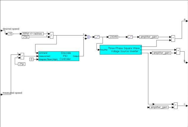
Flip the Rotary Encoder and Hall Sensor blocks using the Edit > Flip Horizontal command. Then arrange the blocks and wire them together, as shown below.

Connect the Hall Sensor outputs to the corresponding inputs of the Brushless PWM Servo Amplifier. Then, wire the output of the PID Controller (Digital) to the reference velocity input of the Brushless PWM Servo Amplifier. Finally, connect the displacement output of the Rotary Encoder to the measurement input of the PID Controller (Digital).

Two const blocks are fed into the Brushless PWM Servo Amplifier; another const block is fed into the PID Controller (Digital):

Set the value of the const block, wired into inhibit, to 1. This prevents inhibit.

In this application, there is no reason to reset the integration of the PID Controller (Digital), so a 0 const is wired to Integrator Reset (High) to disable. In other applications, repetitive control may be used, and Integrator Reset (High) may be required to re-initialize the control between repetitions.

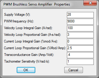
A value of 100 amps is chosen for this example to make certain saturation does not occur. Later on, you might possibly measure currents encountered in this simulation under highest load conditions and set a more appropriate current limit for the final design.

Next, place the following eMotor blocks in the diagram:

•      Brushless DC (BLDC/PMSM) Motor

•      Rotary Encoder

•      Rotational Load

Flip the Rotary Encoder and Rotational Load blocks using the Edit > Flip Horizontal command. Then arrange the blocks to the right of the previous construction, as shown in the following diagram:

The rotor output displacement of the Brushless DC (BLDC/PMSM) Motor connects to three other block connections: the displacement input of the Hall Sensor block, the input of the Rotary Encoder, and the rotary displacement input of the Rotational Load.

Connect the outputs of the PWM Brushless Servo Amplifier to the corresponding inputs of the Brushless DC (BLDC/PMSM) Motor. Connect the load reaction torque vector output connector on the Rotational Load to the load reaction vector input of the Brushless DC (BLDC/PMSM) Motor.

Lastly connect a const block with 0 set value to the load disturbance input connector on the Rotational Load. If there were other torques related to influences that could not be directly represented by the set parameters of the rotary load model, the load disturbance input provides a method for introducing such torques. For the target tracker, it might be conceivable to introduce torque noise induced by structural vibrations of the tracker mount. If the mount were part of a satellite payload, such vibrations could arise from solar array positioning systems. Noise profiles with specific power spectral densities can be generated in Embed using the Random Generator blocks and transferFunction block. Coefficients of the transfer function are determined by applying spectral factorization techniques to the known PSD.

Next, insert a Park Transform and a Clark Transform into the diagram and connect them as shown below:

Encapsulate the blocks in Current Sense. Then label the input and output connector tabs as shown below:

Flip the block 180^o and connect the ias and ibs output connectors of the Brushless DC (BLDC/PMSM) Motor to the corresponding a and b inputs of the Current Sense. Connect the displacement output of the Rotary Encoder to the angle input of the Current Sense. Connect the load displacement output of the Rotational Load to the displacement input of the other Rotary Encoder.

Complete the wiring by connecting the output of the Current Sense to the current sense input of the PWM Brushless Servo Amplifier and the rate output of the Rotary Encoder to the tach input of the PWM Brushless Servo Amplifier, as shown below:

This block construction represents a cascade control loop. The inner loop senses and controls current; the middle loop senses and controls velocity; and the outermost loop senses and controls position.

Now the entire block construction must be captured within a single compound block named X Axis Servo. Reduce the number of inputs and outputs on X Axis Servo to one, and label the input commanded LOS and output actual LOS.

Next, drill into X Axis Servo and make certain that the commanded LOS is connected to the command input of the PID compensator block and the displacement output of the Rotational Load is connected to the actual LOS output of the compound block.

While still in the X Axis Servo, open the dialog boxes of each eMotor block and enter the following parameter values as specified by the design input.

PID Controller (Digital) block

PWM Brushless Servo Amplifier block

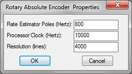
Rotary Encoder block that feeds back to PID Controller (Digital) block

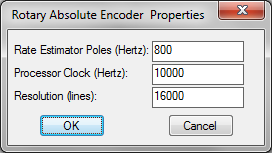
Rotary Encoder block that feeds back into the PWM Brushless Servo Amplifier block

Brushless DC (BLDC/PMSM) Motor block

Rotational Load block

This completes the x-axis of the servo controller. Completing the y-axis takes only a couple of keystrokes, as all dynamics for this axis are assumed to be equal. Make a duplicate copy of X Axis Servo using the Edit > Copy command. In the dialog box for the newly-created X Axis Servo, change the name of the block to Y Axis Servo. At this point, there are two servo controllers in your diagram: an x-axis and a y-axis servo controller.

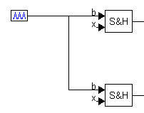
Next, create a simulation of the pipeline image processor. For this processor, the dominant feature is the sample frame rate of 60 Hz. Place two sampleHold blocks (located under Blocks > Nonlinear) and a pulseTrain block (located under Blocks > Signal Producer) in your diagram. Arrange these blocks as shown below:

In the pulseTrain block, set the time between pulses to 1/60 (0.0167). Then encapsulate the three blocks in a compound block Focal Plane Pipeline Processor.

Next, create the following block configuration:

This construction is used to create an elliptical motion for the target in the X-Y plane. Frequency for each axis is the same (1 rad/sec); however, phase differs.

The integrator (1/S) and sin blocks are located under Blocks > Integration and Blocks > Transcendentals, respectively.

Enclose this construct in a compound block and name it Target:

Connect the compound blocks as shown in the following diagram:

In this construction, command line of sight (LOS) is set to the target angle that is determined by the pipeline processor. The difference between the target angle and actual line of sight is calculated using summingJunction blocks that provide focal plane error. The error is converted into degrees using unitConversion blocks.

Setting up the plot blocks

Next, plot blocks are prepared to display simulation output.

Place a plot block (located under Blocks > Signal Consumer) in the diagram; then open its dialog box and under the Options tab enter the following settings:

Note that the Multiple XY Traces parameter is activated. This feature allows the display of the target motion independently from the servo line of sight.

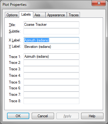
Under the Labels tab, enter the information shown below.

And under the Axis tab, enter the following information:

Place another plot block in the diagram and enter the same parameters as in the previous plot with these exceptions:

Under the Labels tab, make these changes:

•      In the Title box, enter Focal Plane

•      Enter degrees as units instead of radians

•      Under the Options tab, make these changes:

•      Activate Fixed Bounds

•      De-activate Multiple XY Traces

•      Under the Axis tab, make these changes:

•      In X Upper Bound and Y Upper Bound, enter 5

•      In X Lower Bound and Y Lower Bound, enter –5

Setting the simulation properties

Simulation properties are set through the System > System Properties command. Enter the following information to the System Properties dialog box.

For this simulation, a very small step size is necessary because pulse width modulation is being simulated at 9000 hertz.

Final configuration requirements

Connect the X and Y outputs of Target to the first two input tabs of the Coarse Tracker plot block and the outputs of X Axis Servo and Y Axis Servo actual line of sights to the next two input tabs of the same plot block.

Connect the outputs of the two unitConversion blocks to the first two input connectors of the Focal Plane plot.

You are now ready to run the simulation with the System > Go command.

Simulation results

The following plot shows the acquisition and tracking of the actual target’s elliptical motion with the servo line of sight:

To better illustrate accuracy, the following plot shows the focal plane error. The darkened circular area represents the time after the servo has acquired the target and begins tracking. These results show errors to be on the order of 1^o, exceeding the requirement.

It should be noted that to get to this level of control required tuning of each of the control loops with multiple iterations before an acceptable control was achieved.