
Because integration is a more numerically stable operation than differentiation, you need to transform your ordinary differential equations into ones that use integration operators.
To enter an ordinary differential equation in Embed, first algebraically solve the equation for the highest derivative. Then insert the number of integrator blocks that equals the order of the highest derivative. Most continuous systems contain one or more differential equations. For example, if you're solving a third order differential equation, insert three integrator blocks and supply the equation for the highest order derivative as input to the first integrator block. The output of the first integrator is:
which is the next lower order derivative.
The output of the second integrator block is:

and so on. The outputs of the lower order derivatives can be fed back into the calculation of the highest derivative.
The following example steps you through the process of converting a second order differential equation into block diagram form. This example involves the ubiquitous damped harmonic oscillator, where a mass M is suspended from the ceiling by a spring-damper arm. The mass is attracted back toward the origin by an elastic restoring force proportional to its vertical displacement and is damped by an opposing force that acts in proportion to its velocity.
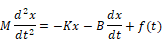
Based on Newton’s Second Law, the definition of the equation of motion for the damped harmonic oscillator is:
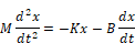
where:
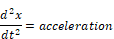

Because integration is inherently more numerically stable than differentiation, the equation must be expressed in terms of integrals. By definition of the derivative:
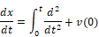
and

where:
v(0) = initial velocity of the mass
x(0) = initial starting position of the mass
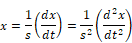
Employing 1/s as the operator for integration, and making the initial conditions implicit in 1/s, yields the following relationship:
The relationship can be expressed in Embed block diagram form as:

A more concise representation of this relationship is:

The three variable blocks hold the quantities d2x/dt2, dx/dt, and x at each instant of time. The variable blocks are extraneous, because the wires alone can carry the data forward to the next block.
Returning to the original equation of motion and solving for the acceleration yields:
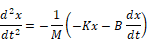
To model this system in Embed, wire the outputs of the x and dx/dt variables through two gains (which represent K and B) and into a summingJunction, with inputs negated. By dividing the output of the summingJunction by M (which is represented by a const), you produce d2x/dt2. Letting K = 5, B = 1, and M = 10, for example, results in the diagram shown below:
This diagram represents a closed-loop system from which the values for position, velocity, and/or acceleration can be displayed in a plot block. The initial conditions of starting position x(0) and velocity v(0) of M are specified within the integrator blocks preceding their respective variable blocks.
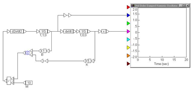
Letting x(0) = 0 and v(0) = 1, and setting the simulation range from 0 to 20 and the step size to 0.05 yields the following results:
Note that the characteristic decay that is observed depends on the parameters M, K, and B. Different values for these quantities and initial conditions can be entered into the appropriate blocks to simulate any system.
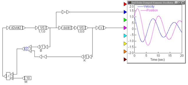
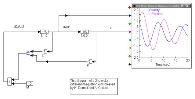
You can simplify the diagram by replacing the variables that denote x, dx/dt, and d2x/dt2 with optional label blocks.
Other physical effects can now be added, such as static and sliding friction, or external driving forces.
A coupled system can also be modeled by interconnecting two separate block diagrams. This permits extremely complex systems to be modeled without the need for a closed mathematical solution.
A transfer function is a ratio of polynomials in the Laplacian s operator that models the ratio of the output signals divided by the input signals. There are two ways to enter a transfer function in Embed. The more common method is via the transferFunction block, which you use when entering coefficients as numeric constants.
When the coefficients are polynomial constants, begin by defining the transfer function in operator notation. The transfer function should be proper; that is, the highest degree of the denominator polynomial m must be greater or equal to that of the numerator n. The general transfer function representation is:
You represent this in Embed as follows:
This diagram represents the condition in which the numerator and denominator degrees are equal (m = n). When the numerator is of a degree less than the denominator, the output paths are removed from the left. For example, if n is two less than m, the an and an-1 output paths would be removed.
Note also that for each kth polynomial term, you add an integrator block and a corresponding ak, bk set of gain blocks that flow to the upper and lower summingJunction blocks in the diagram.
The second-degree transfer function is:
The diagram for this transfer function is:
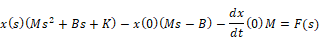
In this system, a vertical draft is produced by a strong fan positioned below the mass. This driving force sustains the motion of the damped oscillator and represents an input to the system. The output is the instantaneous velocity v of the mass. To derive the transfer function for this simple system, you will use the Laplace transform. The modified equation of motion for this system is:
Accounting for non-zero initial conditions, the Laplace transform becomes:

Regrouping the equation yields:
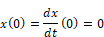
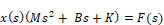
Transfer function representation requires all initial conditions be equal to zero, specifically:
The equation reduces to:
whose transfer function is:
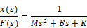
Since velocity rather than displacement is the desired output, the substitution:

is made to produce the transfer function:
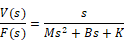
The denominator remains unchanged; however, the numerator coefficients are different. The block diagram becomes:
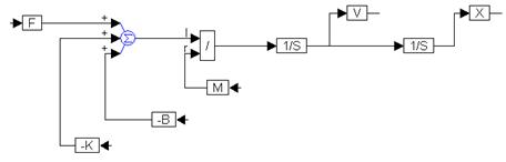
The non-zero initial conditions can be easily included by specifying their values on each of the two integrator blocks. For example, suppose that the spring was initially stretched one inch. An initial condition of one would be placed on the rightmost integrator. Assuming an initial velocity of zero, the initial condition on the leftmost integrator would still be zero.
Consider:

The bilinear transformation can be implemented by the substitution:

The above transfer function becomes:
Embed automatically simplifies this representation and enters the appropriate coefficients for the numerator and denominator polynomials.
It is important to note that in both transformations, the results obtained are dependent on the sampling interval dT. In other words, for a given continuous or discrete transfer function, an infinite number of equivalent discrete or continuous transfer functions may be obtained by varying the sampling interval dT.
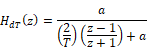
Consider:

The bilinear transformation can be implemented by the substitution:

The above discrete transfer function becomes:
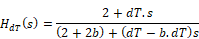
Embed automatically simplifies this representation and enters the appropriate coefficients for the numerator and denominator polynomials.
It is important to note that in both transformations, the results obtained are dependent on the sampling interval dT. In other words, for a given continuous or discrete transfer function, an infinite number of equivalent discrete or continuous transfer functions may be obtained by varying the sampling interval dT.