To generate the transfer function information
•Choose Analyze > Transfer Function Info.
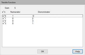
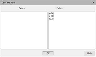
The numerator and denominator coefficients, and the zeros and poles are displayed in successive dialog boxes.
|
|
|
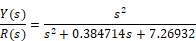
The input to the system is the 0 constant (denoted as R), and the output is the dx/dt signal (as previously defined). The first dialog box presents the transfer function as numerator and denominator polynomials in power of s. Denoting the output as:

the transfer function is:
The gain (s = 0 gain) is 0 by inspection.
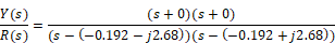
The second dialog box presents the factors of both polynomials. The zeros are the roots of the numerator, and the poles are the roots of the denominator. At this operating point, the system has two real zeros and a complex conjugate pair of poles. The factored transfer function can be expressed as:
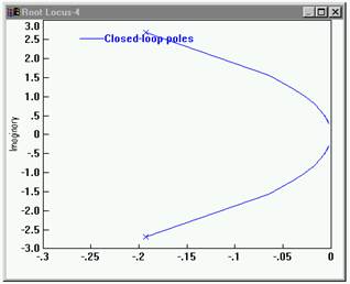
To generate the root locus plot
1. Choose Analyze > Root Locus.
2. Resize and move the plot for easier viewing.
3. Choose Edit > Block Properties.
4. Click over the root locus plot.
5. Click Read Coordinates.
The root locus plot reappears with crosshairs and status bar.
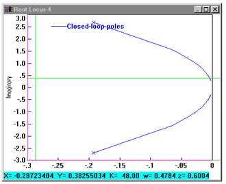
6.
At the selected point, a gain of 48 in feedback around the transfer function
results in a well-damped  rapid responding system
with:
rapid responding system
with:
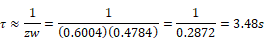
•A time constraint of
•A zero steady-state step error due to the integration at the origin.
Bode plots are frequently used to determine the performance characteristics of a closed-loop system in the frequency domain.
1. Choose Analyze > Frequency Range.
2. In the Bode Frequency Range dialog box, do the following:
•In the Start box, enter 0.1.
•In the End box, enter 10.
•In the Step Count box, enter 100.
3. Choose Analyze > Frequency Response.
4. Resize and move the plots for easier viewing.
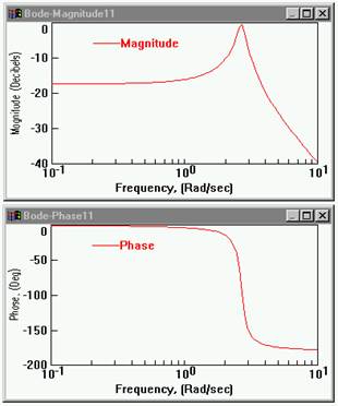
5. To determine the resonant frequency of the magnitude plot, invoke the plot crosshairs:
a. Choose Edit > Block Properties and click the Bode magnitude plot.
b. Select Options and choose Read Coordinates.
The Bode magnitude plot reappears with crosshairs and a status bar.
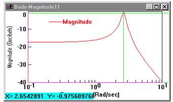
The digital display of the magnitude plot reveals the x coordinate is 2.654 rad/s, the resonant frequency of the system. Note that this value agrees, within the granularity of the digital read-out, with the factored transfer function value of 2.68 rad/s (as solved earlier).