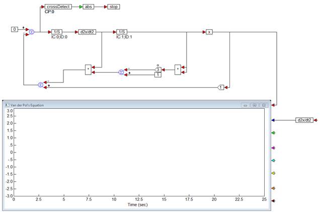
To linearize the system about a specific operating point
An interesting operating point about which to linearize the system is when the d2x/dt2 signal is equal to 0. At this point, the linearization results in stable poles.
1. Wire a crossDetect block to the d2x/dt2 signal.
2. Feed the output into an abs block, which is wired to a stop block.
3. Wire the d2x/dt2 signal into the plot block.

In this configuration, the simulation is automatically stopped when the d2x/dt2 signal is exactly 0. The crossDetect block outputs 1 or -1 depending on whether the crossing occurs with a positive or negative slope. Since the stop block stops the simulation only when the input is 1 or greater, an abs block is introduced between them to ensure that the stop block receives only positive inputs.
4.
Choose System > Go, or click the  toolbar button.
The simulation runs to the first occurrence of signal d2x/dt2 = 0.
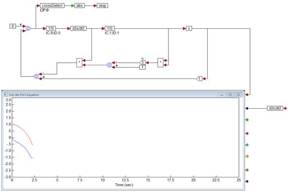
5.
Choose System > Continue, or click  toolbar button to continue the simulation
to the next occurrence of d2x/dt2 = 0.
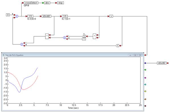
To linearize the system
1. Select the block set to be analyzed. The block set includes all but the 0 input const block and the plot block.
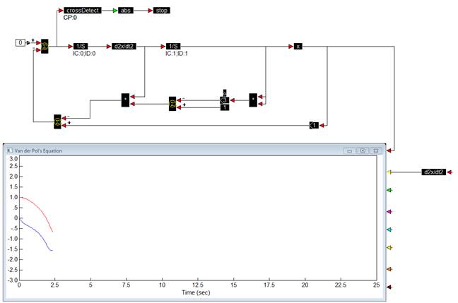
2. Choose Analyze > Select Input/Output Points to specify the reference points for the linearization.
3. Point to the output connector tab on the 0 input const block and click.
4. Point to the input connector tab on the plot block to which the d2x/dt2 signal is wired and click.
5. Point to empty screen and click.
6. Choose Analyze > Linearize.
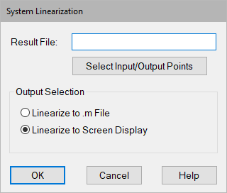
7. Do one of the following:
•To display the ABCD matrices in four separate, successive dialog boxes, select Linearize To Screen Display.
•To write the matrix information to an M file, select the Linearize To .M File and enter a file name in the Result File box. For this example, the contents of the file will be:
function [a,b,c,d] = vabcd
a = [-.384714
-7.26932;
1 0 ];
b = [1 ;
0
];
c = [-.384714 -7.26932];
d = [1 ];