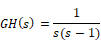
Another example of a type 1 system is the open-loop transfer function:
as shown below:
To generate the Nyquist plot
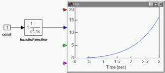
1. Create the above diagram using a const, transferFunction, and plot block.
2. Enter the following polynomial coefficients to the transferFunction block:
Numerator: 1
Denominator: 1 -1 0
Note: Always leave spaces between coefficient values.
3.
Choose System > Go, or click  in the toolbar to simulate the diagram.
4. Select the transferFunction block.
5. Choose Analyze > Nyquist Response.
6. You are reminded that the system has poles on the imaginary axis, which will result in Nyquist circles at infinity. Click OK, or press ENTER.
7. In the Nyquist dialog box, you have the option to change the maximum frequency range. The default value is 10. Leave it unchanged and click OK, or press ENTER.
8. The Nyquist plot appears.
9. Drag on its borders to adjust its size.
In this case, you can observe that the point (-1,0) is enclosed by the Nyquist contour. Consequently N > 0. Moreover, since the number of clockwise encirclements of the point (-1, 0) is one, N = 1. The poles of GH(s) are at s = 0 and s = +1, with the second pole appearing in the right-half plane. This implies that P, the number of poles in the right-half plane, equals one.
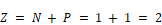
In this case, N ≠ -P, which indicates that the system is unstable.
The number of zeros of 1 + GH(s) in the right-half plane is given by: