Setting up the integration algorithm involves choosing the algorithm, and, if you choose an adaptive algorithm, specifying the minimum step size, error tolerance, and iteration count.
Embed provides seven integration algorithms — Euler, trapezoidal, Runge Kutta 2nd order, Runge Kutta 4th order, adaptive Runge Kutta 5th order, adaptive Bulirsh-Stoer, and backward Euler (Stiff) — of varying numerical accuracy for the numerical integration of differential and difference equations.
Each algorithm provides a numerical approximation to continuous integration. The approximation is based on a trade-off between speed of execution and accuracy. Generally speaking, the more complex algorithms yield more stable and numerically correct results; however, they also take longer to run.
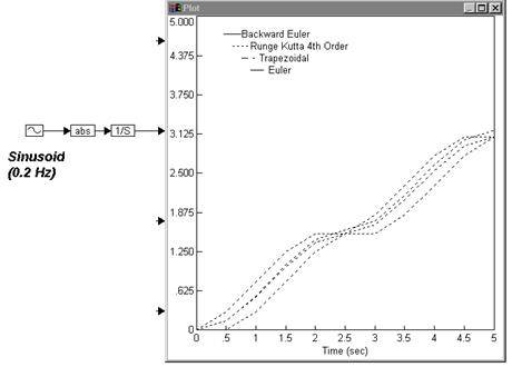
For example, the integration of the absolute value of a sinusoid signal with a frequency of 0.2 Hz is plotted below. The output of the abs block is a sequence of sinusoid positive half-cycles with a frequency of 0.4 Hz. Since the simulation range is from 0 to 5 sec, the output of the integrator block is the estimate area under the curve of two positive half-cycles.
While the differences due to the integration algorithms are negligible for this example, more dramatic differences can be observed when comparing simulation methods in diagrams containing differential equations.
A good rule of thumb, then, is to use the least complicated algorithm that provides stable and correct results. To achieve this, start with the most complex integration algorithm and work backwards to simpler algorithms until you see a noticeable change in your results.
If you plan on using a particular integration algorithm a lot, you can set it as a default as described under Setting simulation defaults.
To set the integration method
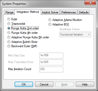
1. Choose System > System Properties.
2. Click the Integration Method tab.
3. Choose the options you want, then click OK, or press ENTER.
Absolute Tolerance: When you select Adaptive Adams-Moulton or Adaptive BDF, you can specify the absolute tolerance. If the estimated error is greater than the specified absolute tolerance, the adaptive time step algorithm will attempt to improve the solution accuracy by reducing the time step.
Adaptive Adams-Moulton: Allows you to specify Newton iteration for stiff systems and Function Iteration for non-stiff systems. For stiff systems, adaptive Adams-Moulton provides more accurate solutions: it detects discontinuities and automatically shrinks the step size around them.
Adaptive BDF: Allows you to specify Newton iteration for stiff systems and Function Iteration for non-stiff systems. For stiff systems, adaptive BDF provides more accurate solution: it detects discontinuities and automatically shrinks the step size around them.
Adaptive Bulirsh-Stoer: Uses rational polynomials to extrapolate a series of substeps to a final estimate. This algorithm is highly accurate for smooth functions.
Adaptive Runge Kutta 5th order: Obtains fifth order accuracy. This algorithm automatically takes small step sizes through discontinuities in the input function and large strides through smooth functions.
Backward Euler (Stiff): Obtains efficiency for systems with high and low frequencies. The other algorithms would require small step sizes to maintain stability.
Euler: Evaluates once per simulation time step. This method is least affected by singularities, and is fastest for moderate step sizes.
Max Iteration Count: When you select an adaptive integration algorithm, you can also specify the maximum number of times the integration algorithm will vary its time step attempting to meet the maximum truncation error criterion. The default value for the maximum iteration count is 5.
Min Step Size: The adaptive Runge Kutta 5th order and adaptive Bulirsh-Stoer integration algorithms exert more control over the accuracy of the solution by letting you specify a minimum step size. The step size is continually adjusted to meet the error tolerance and iteration count criteria; however, it is never reduced below the minimum step size. Thus, inaccurate results may be produced if the minimum step size is too large, the error tolerance is too large, or the iteration count is too small.
The default value for the minimum step size is 1e-006.
Nonlinear Solver: When you select Adaptive Adams-Moulton or Adaptive BDF, you have a choice of nonlinear solver:
•Functional Iteration: Generalized Minimal Residual method, or GMRES with scaling and preconditioning.
•Newton: For stiff systems, Newton iteration is used. This requires the solution of linear systems of the form by approximating the Newton matrix I -hBn,0J where J is the ODE system Jacobian (df/dy).
Relative Tolerance: When you select Adaptive Adams-Moulton or Adaptive BDF, you can specify the relative tolerance. If the ratio of the estimated error is greater than the specified relative tolerance, the adaptive time step algorithm will attempt to improve the solution accuracy by reducing the time step.
Runge Kutta 2d order: Obtains second order accuracy. This method uses a midpoint step derivative to calculate the final integration value. Specify the length of the step in the Step Size box.
Runge Kutta 4th order: Obtains fourth order accuracy. This method evaluates the derivative four times at each time step: once at the initial point, twice at sample midpoints, and once at a sample endpoint. The final integration value is then derived based on these derivatives.
Trapezoidal: Evaluates twice per simulation time step.