transferFunction

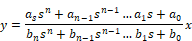
Description: The transferFunction block executes a single-input single-output linear transfer function specified in the following ways:

• As an M file created with Embed: The Linearize command in the Analyze menu generates ABCD state-space matrices from the nonlinear system by numerically evaluating the matrix perturbation equations at the time the simulation was halted.

• As an M file created with a text editor: The following is an example of a user-written M file:

• As a MAT file created with MATLAB: Generating MAT files is described in the MATLAB documentation. Note that when you save the abcd matrices to file, the names of the matrices are not important; however, the order in which they appear is.

When you simulate the block diagram, Embed numerically solves the transferFunction block. The transferFunction block’s Properties dialog box allows you to control how the numerator and denominator polynomials are entered.

Code Generation: When generating code for C2000 or ARM Cortex targets and you include one or more transferFunction blocks in your diagram and you activate Check for Performance Issues in the Code Generation dialog box, Embed warns you that large RAM blocks are not supported for the target. You can continue with code generation; however, the generated code may not fit in the target RAM and the code will run slower.

When generating code for Arduino or MSP430 targets, you cannot include transferFunction blocks in your diagram. Embed halts code generation and issues a message to replace the block.

Discrete transfer function: To implement a discrete transfer function, activate the discrete parameter and enter the discrete coefficients directly to the Numerator and Denominator parameters. Conversely, you can enter continuous coefficients and then press Convert S->Z to perform a Tustin transform of S to Z domain.

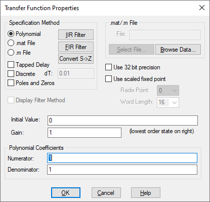
Display Filter Method Displays the filter specification on the block. When Display Filter Method is not activated, Embed displays the polynomial coefficients.

Gain: Indicates the transfer function gain. If the leading terms of the numerator and denominator coefficients are not unity, Embed will adjust the gain to make it so. The default value is 1.

Initial Value: Specifies initial values for the states in the block. The values are right-adjusted. The right-most value corresponds to the lowest order state. Unspecified states are set to 0. The initial value can be a variable.

.mat/.m File: Lets you specify the name of the M or MAT file to be used as input to the transferFunction block. If you do not know the name, click Select File to find it.

Polynomial Coefficients

Denominator: Indicates the denominator polynomial for the transferFunction block. Separate values with a space. Embed determines the order of the transfer function by the number of denominator coefficients you enter. For example, an nth order transfer function will have n + 1 coefficients. You can specify the denominator as a matrix expression.

Numerator: Indicates the numerator polynomial for the transferFunction block. Separate values with a space. You can specify the numerator as a matrix expression.

Specification Method

Discrete: Indicates a discrete Z-Domain transfer function. Enter the coefficients directly into the Numerator and Denominator parameters. Enter the time step for the discrete transfer function in the dT box. By default, Embed uses the step size established with the System > System Properties command. When Discrete is de-activated, a continuous transfer function is created. For information on resolving issues with discrete transfer function behavior, see the Embed discrete transferFunction Forum entry.

dT: Specifies the time step for the discrete transfer function. By default, Embed uses the step size parameter from the System > System Properties command.

Poles and Zeros: Lets you enter a transfer function via zeros and poles in the Numerator and Denominator boxes, respectively. Enter each root in the following format:

(real-part, imaginary-part)

For large order systems, poles and zeros is more numerically accurate.

Polynomial: Indicates that the transfer function is to be specified as numerator and denominator polynomials. Supply the numerator and denominator polynomials and gain under the Polynomial Coefficients group box. .mat file indicates that the transfer function is to be specified as a MAT file. Specify the name of the MAT file in the .mat/.m File group box. .m file indicates that the transfer function is to be specified as an M file. Specify the name of the M file in the .mat/.m File group box.

Tapped Delay: Provides tapped delay implementation for high-order FIR filters.

Use 32-Bit Precision: Simulates the behavior of the transfer function at 32-bit precision. Normally, all Embed blocks are 64-bit precision. This parameter allows you to simulate the effect of code running on a floating point 32-bit target.

Use Scaled Fixed Point: When targeting a fixed-point processor, such as a TI C2000, activate this parameter. Embed uses scaled fixed-point internal operations and will generate scaled fixed-point code.

Convert S to Z button: Uses bilinear transformation to convert a continuous transfer function to an equivalent discrete transfer function with a sampling interval of dT.

Convert Z to S button: Uses bilinear transformation to convert a discrete transfer function to an equivalent continuous transfer function.