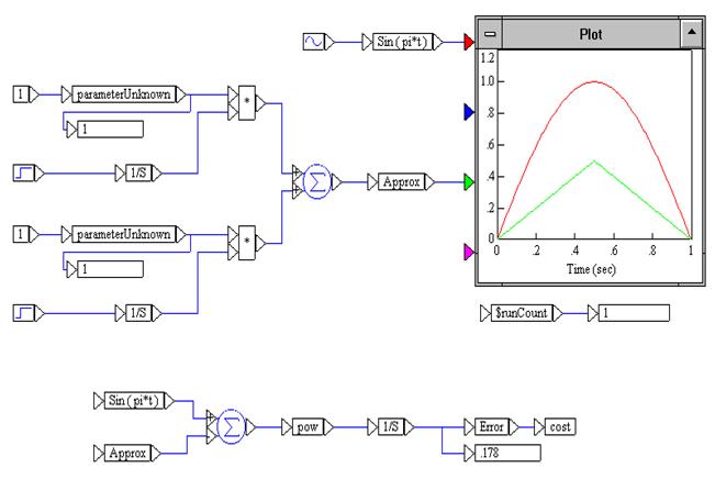
When you open CURV2P, the following diagram appears on the screen:

The function Sin (πt) is produced by a sinusoid block with frequency π and amplitude 1. It is wired into a variable block labeled Sin ( pi*t ). The approximating function is produced with two step blocks and two integrator blocks. This function is wired into a variable block labeled Approx. Both curves are plotted.
The cost or objective function is computed by integrating the squared difference of the two curves, (Sin ( pi*t ) - Approx)2 , from 0 to 1. The error is wired into a cost block to identify it as the objective function.
Each of the parameterUnknowns is wired to a const block with value 1. This provides starting values for the parameterUnknowns or decision variables. A simulation run plots the two curves and computes the error for the starting values as 0.178.
To find the best multipliers for the approximating function to produce the smallest error, the multipliers are wired to parameterUnknown blocks (which alert Embed that optimization may be performed on these decision variables) and then into a display block so that the parameters can be monitored during the optimization run. Upper and lower bounds of 10 and -10 have been set for these parameters in the parameterUnknown blocks. To view or change the bounds, right-click the parameterUnknown block.