Creating a Braided Cable Shield Layer (Vance, Tyni or Demoulin)

Create a single layer, braided (Vance, Tyni, Demoulin) cable shield. For a braided shield layer, the relevant braid parameters and weave metal are specified and the Solver determines the frequency-dependent impedance (Zs + Zt) and admittance (Yt) matrix using the Vance, Tyni or Demoulin formulation.

1. On the Cables tab, in the Definitions group, click the  Cable shield icon.
2. Under Shield layer(s), click Single to create a single-layered shield.
3. On the Inner layer tab, on the Impedance definition tab, from the Definition method drop-down list, select one of the following:
   • Braided (Vance)
   • Braided (Tyni)
   • Braided (Demoulin)

   
   

   

   
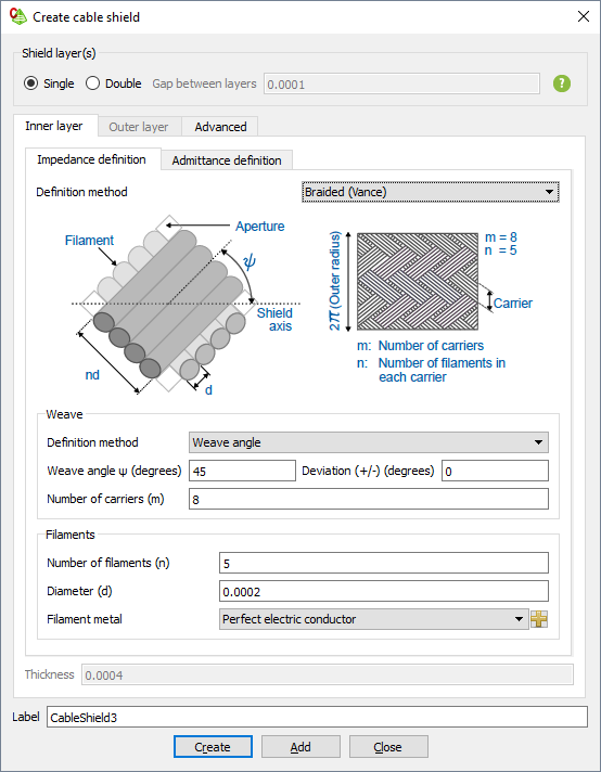
   Figure 1. The Create cable shield dialog.

4. Under Weave, specify the following:
   1. From the Definition method drop-down list, select Weave angle to create a braided layer using the weave angle definition:
      • In the Weave angle (degrees) field, enter a value in degrees for the nominal weave angle.
      • In the Deviation (+/-) (degrees) field, enter a value for the deviation of the weave angle from the nominal weave angle in degrees.
   2. From the Definition method drop-down list, select Optical coverage to create a braided layer using the optical coverage definition:
      • In the Minimum optical coverage (%) field, enter a percentage for the minimum optical coverage for the braided layer.
   3. In the Number of carriers (m) field, specify the number of carriers in the braided layer.
5. Under Filaments, specify the following:
   1. In the Number of filaments (n) field, enter a value for the number of filaments in a single carrier.
   2. In the Diameter (d) field, enter a value for the filament diameter.
   3. In the Filament metal drop-down list, select one of the following:
      • To create a filament consisting of PEC, select Perfect electric conductor.
      • To create a filament consisting of a predefined metal, select the metal.
      • To create a filament consisting of a metal, which is not yet defined in the model, select the icon to define a metal or add a metal from the media library.

6. On the Inner layer tab, on the Admittance definition tab, select Same as impedance definition, from the Definition method drop-down list to use the Vance, Tynior Demoulin formulation for the admittance matrix.

   
   

   

   
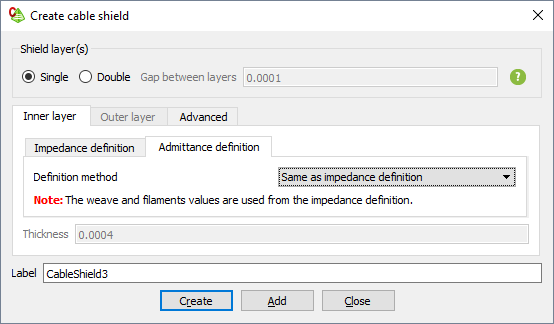
   Figure 2. The Create cable shield dialog.

   Note:

   The weave and filaments values are used from the impedance definition to calculate the admittance matrix.

7. In the Label field, add a unique label for the cable shield.
8. Click Create to create the cable shield and close the dialog.