Optimising the Bandpass Filter with HyperStudy Using Scripting
Configure the HyperStudy setup and perform the optimisation. Minimize the reflection coefficient.
-
Under the Study group, click
New.
The Add Study dialog is displayed.
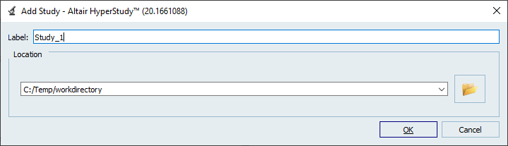
Figure 1. The Add Study dialog. -
Click in the Explorer tab.
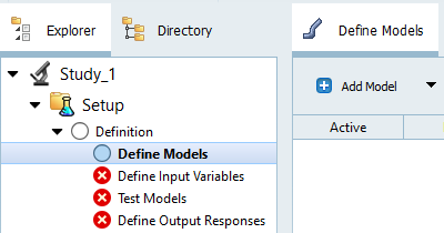
Figure 2. Example of the Study tree in HyperStudy. -
Click Add Model.
The Add dialog is displayed.
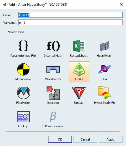
Figure 3. The Add dialog. -
Click Import Variables to import CADFEKO model variables.
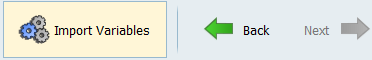
Figure 4. Example selecting the Import Variables button. -
Select which variables to include in the study. Only S1 – S3 should be
activated and the default ranges used.
An example of the selected variables is displayed.
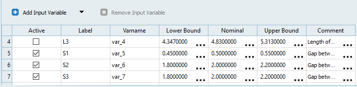
Figure 5. Example of the variable selection -
Click Run Definition.
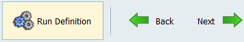
Figure 6. Example selecting the Run Definition button.During the Write phase, the bandpassfilter.cfx_extract.lua file was copied to the run directory and executed after the Feko solver was run in the Extract phase. This generated an output file that HyperStudy can process easily.Note: The script bandpassfilter.cfx_extract.lua is different if a .pfs file was present before importing the variables and will automatically extract the visible traces on a Cartesian graph and polar graph.See Figure 7 for the completed definition run for the Write, Execute and Extract phases for the initial test run done by HyperStudy.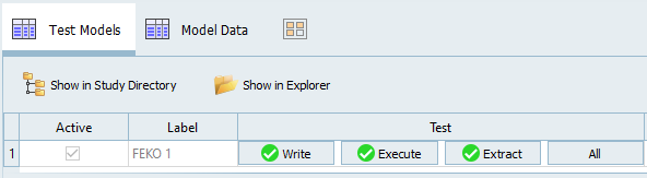
Figure 7. Example of the completed definition run. -
Click File Assistant.
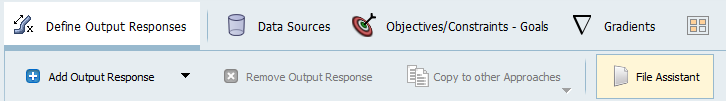
Figure 8. Selecting the File Assistant button.The File Assistant dialog is displayed.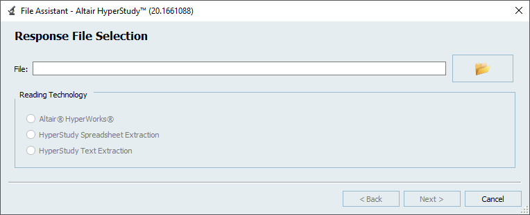
Figure 9. The File Assistant dialog. -
Confirm that Single Item in a Time Series is selected
and click Next.
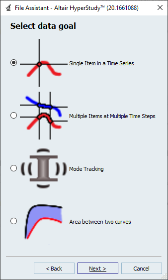
Figure 10. The File Assistant dialog. -
Confirm that s11avg is selected and click
Next.
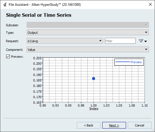
Figure 11. The File Assistant dialog. -
In the Label field, enter s11avg
to change the name of the response label.
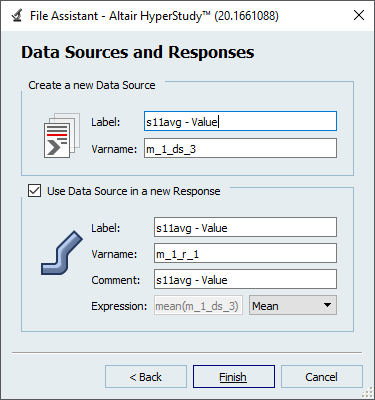
Figure 12. The File Assistant dialog. -
Under Goals click
 to add an optimisation goal.
The following dialog is displayed.
to add an optimisation goal.
The following dialog is displayed.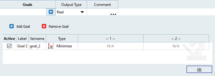
Figure 13. Example adding an optimisation goal. -
Click Evaluate to extract the value from the output
file.
Figure 14. Example selecting the Evaluate button.HyperStudy is now configured to understand which model to use, which variables are available for modification and how to process the output. -
Right-click on the defined study in the Explorer tab and
click Add.
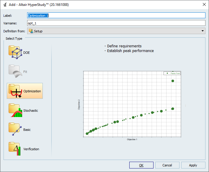
Figure 15. The Add dialog and selecting an optimisation approach. -
In the Definition from:
drop-down list, select Setup and click OK
The optimisation approach is created in the Explorer tab
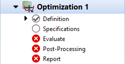
Figure 16. Example of the Optimisation 1 approach created. -
Click , and select the Adaptive Response Surface
Method as the optimiser.
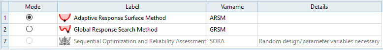
Figure 17. Selecting the Adaptive Response Surface Method. -
Click Apply and click Next.
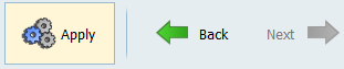
Figure 18. Example selecting the Apply button. -
Click Evaluate Tasks.
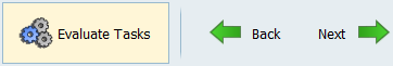
Figure 19. Example selecting the Evaluate Tasks button.Each of the input variables is altered randomly, and its effect on the response analysed.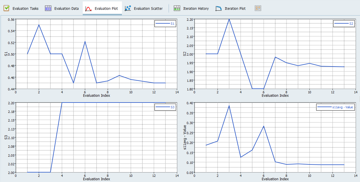
Figure 20. Typical progress data for an ARSM optimisation.