Introduction of background knowledge regarding flow physics and CFD as well as detailed information about the use of AcuSolve and what specific options do.
Collection of AcuSolve simulation cases for which results are compared against analytical or experimental results to demonstrate the accuracy
of AcuSolve results.
In this application, AcuSolve is used to simulate the flow of water between concentric cylinders. The outer cylinder is held stationary while the
inner cylinder rotates with a constant speed. AcuSolve results are compared with analytical results as described in White (1991). The close agreement of AcuSolve results with analytical results validates the ability of AcuSolve to model cases containing thin annular gaps with flow induced by rotating walls.
In this application, turbulent flow of air through a pipe is simulated. AcuSolve results are compared with experimental results as described in White (1991) and extracted from the Moody chart. The
close agreement of AcuSolve results with experimental results validates the ability of AcuSolve to model turbulent flow within pipes.
In this application, AcuSolve is used to simulate the viscous flow of water between a moving and a stationary plate with an imposed pressure
gradient. AcuSolve results are compared with analytical results described in White (1991). The close agreement of AcuSolve results with analytical results validates the ability of AcuSolve to model cases with imposed pressure gradients.
In this application, AcuSolve is used to simulate the flow of air in an enclosed cylindrical cavity with a rotating top and a fixed bottom.
AcuSolve results are compared with experimental data adapted from Michelsen (1986). The close agreement of AcuSolve results with experimental data validates the ability of AcuSolve to model cases containing enclosed cavities with flow induced by rotating walls.
In this application, AcuSolve is used to simulate natural convection in the annular space between a heated inner pipe and an outer concentric pipe.
AcuSolve results are compared with experimental results adapted from Kuehn and Goldstein (1978). The close agreement of AcuSolve results with experimental results validates the ability of AcuSolve to model cases with flow induced by natural convection.
In this application, AcuSolve is used to simulate laminar flow through a channel with two outlets forming a T-junction. AcuSolve results are compared with experimental results adapted from Hayes and others (1989). The close agreement of AcuSolve results with experimental results validates the ability of AcuSolve to model cases with multiple outlet paths.
In this application, AcuSolve is used to simulate high Peclet number laminar flow through a channel with heated walls. AcuSolve results are compared with analytical results adapted from Hua and Pillai (2010). The close agreement of AcuSolve results with analytical results validates the ability of AcuSolve to model cases involving heat transfer to a moving fluid with a high Peclet number.
In this application, AcuSolve is used to simulate turbulent flow of air through and behind a two dimensional open-slit V. AcuSolve results are compared with experimental results adapted from Yang and Tsai (1993). The close agreement of AcuSolve results with experimental results validates the ability of AcuSolve to model the Coandă effect.
In this application, AcuSolve is used to simulate turbulent flow of a fluid over a NACA 0012 airfoil at 3 angles of attack, 0 degrees, 10
degrees, and 15 degrees. AcuSolve results are compared with experimental results for coefficients of pressure, lift, and drag reported by NASA. The
close agreement of AcuSolve results with experimental results validates the ability of AcuSolve to model external aerodynamics.
In this application, AcuSolve is used to simulate the natural convection of a turbulent flow field within a tall rectangular cavity. AcuSolve results are compared with experimental results as described in Betts and Bokhari (2000). The close agreement of AcuSolve results with experimental results validates the ability of AcuSolve to model cases with natural convection of turbulent flow within a tall cavity.
In this application, AcuSolve is used to simulate the separation of laminar flow over a blunt plate. AcuSolve results are compared with experimental results as described in J.C. Lane and R.I. Loehrke (1980). The close
agreement of AcuSolve results with the experimental results validates the ability of AcuSolve to model cases with external laminar flow including separation.
In this application, AcuSolve is used to simulate fully developed turbulent flow through an asymmetric diffuser with a divergent lower wall and
a straight upper wall. AcuSolve results are compared with experimental results as described in Buice and Eaton (2000). The close agreement of AcuSolve results with experimental results validates the ability of AcuSolve to model cases with internal turbulent flow with flow separation and reattachment in an asymmetric diffuser.
In this application, AcuSolve is used to simulate fully developed turbulent flow through an axisymmetric diffuser with a divergent upper wall and
a straight lower wall. AcuSolve results are compared with experimental results as described in Driver (1991) and on the NASA Langley Research Center
Turbulence Modeling Resource webpage. The close agreement of AcuSolve results with experimental data and reference turbulence model performance validates the ability of AcuSolve to model cases with turbulent flow with separation due to an adverse pressure gradient within an axisymmetric
geometry.
In this application, AcuSolve is used to simulate fully developed turbulent flow over a backward-facing step. AcuSolve results are compared with experimental results as described in Driver (1985) and on the NASA Langley Research
Center Turbulence Modeling Resource web page. The close agreement of AcuSolve results with experimental data and reference turbulence model performance validates the ability of AcuSolve to model cases with turbulent flow that forms a shear layer, recirculates and then reattaches downstream
of the divergent step.
In this application, AcuSolve is used to simulate fully developed turbulent flow through a channel containing a convex curve in the lower wall.
AcuSolve results are compared with experimental results as described in Smits (1979) and on the NASA Langley Research Center
Turbulence Modeling Resource webpage. The close agreement of AcuSolve results with experimental data and reference turbulence model performance validates the ability of AcuSolve to model cases with turbulent flow moving past a convex curved wall.
In this application, AcuSolve is used to simulate the heat transfer due to radiation between concentric cylinders. The inner and outer cylinders
are held at constant temperature and are defined to be radiation surfaces. AcuSolve results are compared with analytical results for temperature as described in Incropera (2006). The close agreement
of AcuSolve results with analytical results validates the ability of AcuSolve to model cases with radiation heat transfer requiring view factor computation.
In this application, AcuSolve is used to simulate the mixing of two streams of fluid with different velocities moving past a splitter plate.
AcuSolve results are compared with experimental results as described in J. Delville, et al. (1989). The close agreement of
AcuSolve results with the experimental results validates the ability of AcuSolve to model mixing layers in the turbulent flow regime.
In this application, AcuSolve is used to solve for the flow field around a high lift airfoil with inflow conditions that lead to transitional flow
on the pressure and suction side of the airfoil's surface. The moderate level of turbulence intensity at the inlet,
low angle of attack and shape of the airfoil induce a transition to turbulent flow after a separation bubble develops
on the surface. The coefficient of pressure is compared against experimental data from laboratory experiments.
In this application, AcuSolve is used to simulate turbulent flow through a strongly curved two dimensional 180 degree U-duct channel. AcuSolve results are compared with experimental results adapted from Rumsey et al. (2000). The close agreement of AcuSolve results with experimental results validates the ability of AcuSolve to model turbulent cases with strong curvature effects.
In this application, AcuSolve is used to simulate the heat transfer due to conduction and radiation between concentric spheres. The inside surface
of the inner and the outside surface of the outer sphere are both held at constant temperature, while the gap between
them radiates the heat from one sphere to the other.
In this application, AcuSolve is used to simulate the heat transfer due to radiation through a specular interface within an absorbing, emitting,
but not scattering solid cube. One of the cube’s walls is modeled with an isotropic external radiation source while
the remainder of the cube is held at fixed temperature conditions and modeled with pure radiation, neglecting the
effects of conduction.
In this application, AcuSolve is used to simulate the wall heat flux due to nucleate boiling at a heated wall inside a rectangular channel with
water flow. Results are compared with experimental heat flux measurements as reported by Steiner, et al. (2005). The
close agreement of AcuSolve results with experimental results validates the ability of AcuSolve to model single phase nucleate boiling problems.
This section includes validation cases that consider unbounded simulation domains where external flow is present over
solid bodies, leading to free boundary layer development.
This section includes validation cases containing conditions producing laminar to turbulent flow that are simulated
with a turbulence transition model.
This section includes validation cases that consider time dependent motion within the domain, requiring that the mesh
movement be modeled with a differential equation, a fully defined mesh motion or by interpolated mesh motion.
Collection of AcuSolve simulation cases for which results are compared against analytical or experimental results to demonstrate the accuracy
of AcuSolve results.
In this application, AcuSolve is used to simulate fully developed turbulent flow through an asymmetric diffuser with a divergent lower wall and
a straight upper wall. AcuSolve results are compared with experimental results as described in Buice and Eaton (2000). The close agreement of AcuSolve results with experimental results validates the ability of AcuSolve to model cases with internal turbulent flow with flow separation and reattachment in an asymmetric diffuser.
Turbulent Flow with Separation in an Asymmetric Diffuser
In this application, AcuSolve is used to simulate fully
developed turbulent flow through an asymmetric diffuser with a divergent lower wall and a
straight upper wall. AcuSolve results are compared with
experimental results as described in Buice and Eaton (2000). The close agreement of AcuSolve results with experimental results validates the ability of
AcuSolve to model cases with internal turbulent flow with
flow separation and reattachment in an asymmetric diffuser.
Problem Description
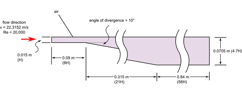
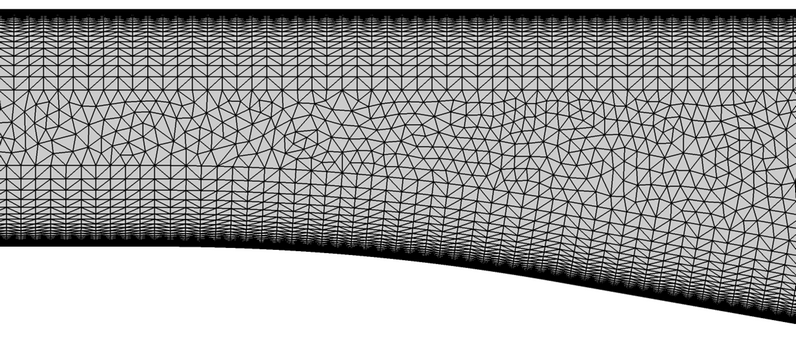
The problem consists of air flowing through an asymmetric diffuser with a divergent lower wall
and a straight upper wall, as shown in the following image, which is not drawn to
scale. The diffuser inlet has a height of 1.5 cm (H) and extends 9 cm (6H) to the
divergent section. The lower wall of the diffuser diverges at an angle of 10° and
expands to 7.05 cm (4.7H). The divergent section has a horizontal length of 31.5 cm
(21H). The expanded section of the diffuser extends 84 cm (56H) to the outlet. Air,
with a density of 1.225 kg/m3 and a viscosity of 1.8325 X 10⁻⁵
kg/m-s enters the diffuser through the inlet of the diffuser with a fully developed
turbulent profile at a Reynolds's number of 20,000. The simulation was conducted
with the Reynolds Averaged Navier-Stokes equations using four turbulence models,
Spalart Allmaras, Shear Stress Transport (SST), K-ω and Realizable K-ε.
The simulation was performed as a two dimensional problem by constructing a volume mesh that
contains a single layer of elements extruded in the cross stream direction
(perpendicular to the flow plane) and by imposing symmetry boundary conditions on
the extruded planes.
AcuSolve Results
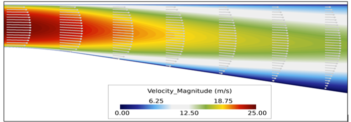
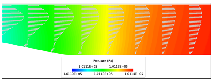
The AcuSolve solution converged to a steady state and the results
reflect the mean flow conditions. As the fully developed turbulent flow enters the
divergent section, the peak velocity is maintained until the expansion of the
cross-sectional height, forms an adverse pressure gradient. After the flow enters
the divergent section, the velocity decreases significantly, due to the expansion of
the cross-section height. This causes separation of the flow along the divergent
wall and results in an area of recirculation. The bulk of the flow above the
divergent wall maintains its streamwise direction, while a portion of it reverses
direction before reattaching further downstream of the divergent section. The
following images show the steady state flow solution for flow within the
diffuser.
Upstream of the diffuser section, the streamline velocity increases as the distance from the
lower wall increases until it reaches the maximum velocity at the center of the
channel. As the flow enters the divergent section of the channel, the streamwise
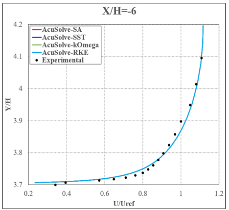
velocity decreases near the bottom wall. The images below show the velocity profiles
at three locations as measured from the midpoint of the curve where the bottom wall
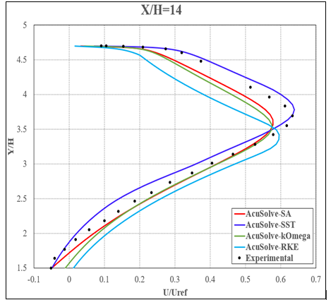
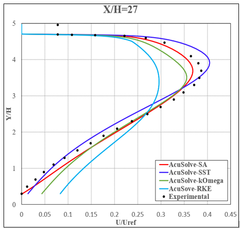
begins to diverge (X=0.0) for each of the tested turbulence models. The first
location, where X/H = -5.944, is close to the inlet. The second location, where X/H
= 13.468, is approximately 0.2 m downstream of the divergent section (~ 0.1 m from
the fully expanded section). The third location, where X/H = 24.066, is
approximately 0.16 m downstream of the point where the diffuser has reached the
maximum height. In these plots the black circles represent the experimental
measurements (Buice and Eaton 2000), the solid red lines for the prediction for the
Spalart Allmaras model, solid blue lines for the prediction for the SST model, solid
green lines for the prediction for the K-ω model and solid cyan lines for the K-ε
model, representing the AcuSolve results. The
non-dimensional height is represented by the fraction of the vertical height (Y)
divided by the inlet height (H) and the velocity is normalized by the inlet velocity
(Uref).
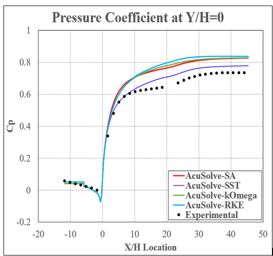
The non-dimensional pressure coefficient (Cp), defined by the integrated inlet pressure and Uref
predicted by AcuSolve along the bottom of the diffuser
is compared to experimental results. The figure below shows Cp, along a constant
vertical height, as a function of the streamwise distance from the inlet of the
channel. The results demonstrate that AcuSolve is
capable of accurately predicting the pressure within the diffuser within the
expected range based on the type of turbulence model used. The performance of the
three turbulence models were found to be consistent with previously published
results for flow through the diffuser as published by Buice and Eaton (2000), with
the SST model predicting the pressure distribution most accurately. Note that the
inlet of the experimental duct was 6H longer than that modeled - AcuSolve values where X/H < -6 are reported as the inlet
value.
Summary
In this application, a fully developed turbulent flow at a Reynolds number of 20,000 is studied. Due to the adverse pressure gradient, separation of flow occurs and causes recirculation in the divergent section of the diffuser. The results were found to be consistent with previously published computational studies and experimental data. The results of this validation demonstrate the ability of
AcuSolve to accurately predict the separation point, the recirculation that occurs along the divergent wall, and the reattachment point in the straight section of the diffuser.
Simulation Settings for Turbulent Flow with Separation in an Asymmetric
Diffuser
HyperWorks CFD database file: <your working
directory>\asymmetric_diffuser_turbulent\asymmetric_diffuser_turbulent.hm
Global
Problem Description
Analysis type - Steady State
Turbulence equation - Spalart Allmaras
Auto Solution Strategy
Max time steps - 150
Relaxation Factor - 0.2
Material Model
Air
Density - 1.225.0 kg/m3
Viscosity - 1.8325e-5 kg/m-sec
Model
Volume
Volume
Element Set
Material model - Air
Surfaces
Bottom
Simple Boundary Condition
Type - Wall
Inlet
Simple Boundary Condition (disabled to allow for nodal boundary
conditions to be set)
Advanced Options
Nodal Boundary Conditions
X-Velocity
Type - Linear
Precedence - 2
Curve fit variable - Y coordinate
Curve fit values (included in database)
Y-Velocity
Type - Linear
Precedence - 2
Curve fit variable - Y coordinate
Curve fit values (included in database)
Eddy Viscosity
Type - Linear
Precedence - 2
Curve fit variable - Y coordinate
Curve fit values (included in database)
Outlet
Simple Boundary Condition
Type - Outflow - 101139.0 Pa
Side 1
Simple Boundary Condition
Type - Symmetry
Side 2
Simple Boundary Condition
Type - Symmetry
Top
Simple Boundary Condition
Type - Wall
References
C.U. Buice, and J.K., Eaton. "Experimental Investigation of Flow Through an
Asymmetric Plane Diffuser". Journal of Fluids Engineering 122:433-435. June
2000.
S. Obi, K. Aoki and S. Masuda. "Experimental and Computational Study of
Turbulent Separating Flow in an Asymmetric Plane Diffuser". Ninth Symposium on
Turbulent Shear Flows. p. 305. Kyoto, Japan. August 16-19, 1993.