HS-1050: Minimization of External Rosenbrock Function

1. Start HyperStudy.
2. Start a new study in the following ways:
   • From the menu bar, click File > New.
   • On the ribbon, click .
3. In the Add Study dialog, enter a study name, select a location for the study, and click OK.
4. Go to the Define Models step.
5. Add a Parameterized File model.
   1. From the Directory, drag-and-drop the appropriate .tpl file into the work area.
      • If you are using Python, use the rosenbrock_py.tpl file.
      • If you are using Compose, use the rosenbrock_oml.tpl file.

      
      
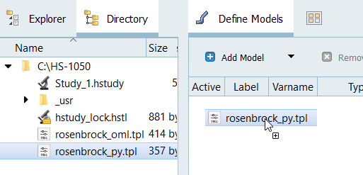
      Figure 1.

   2. In the Solver input file column, enter a name for the solver input file HyperStudy writes during any evaluation.
      • If you are using Python, enter rosenbrock.py.
      • If you are using Compose, enter rosenbrock.oml.
   3. In the Solver execution script column, select either Python (py) or Compose (oml) accordingly.
      Note: If you are using Compose as part of the HyperWorks suite, then HyperStudy should automatically point to the correct .bat file. If you have Compose as separate installation, then during the Register Solver Script step you should point to Compose_batch.bat.
   4. If you are using Compose as the Solver execution script, in the Solver input arguments column, enter -f infront ${file}.
      Note: For solver scripts running on Linux, enter "-f ${file} -nobg" in the Solver input arguments column to ensure that the Compose batch mode runs in the foreground instead of the background.
6. Click Import Variables.
   Two input variables are imported from the .tpl file.
7. Go to the Define Input Variables step.
8. Change both input variable's lower, initial and upper bounds to the values indicated in Figure 2.

   
   
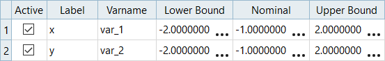
   Figure 2.

1. Go to the Test Models step.
2. Click Run Definition.
   An approaches/setup_1-def/ directory is created inside the study Directory. The approaches/setup_1-def/run__00001/m_1 directory contains the input file, which is the result of the nominal run.

In this step you will create one output responses.

1. From the Directory, drag-and-drop the rosenbrock.res file, located in the approaches/setup_1-def/run__00001/m_1 directory, into the work area.
2. In the File Assistant dialog, set the Reading technology to Altair® HyperWorks® and click Next.
3. Select Single Item in a Time Series, then click Next.
4. Define the following options, and then click Next.
   1. Set Type to unknown.
   2. Set Request to Block 1.
   3. Set Component to Column 1.

   
   
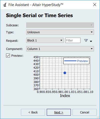
   Figure 3.

5. Optional: Enter labels for the data source and output response.
6. Set Expression to First Element.
   The expression changes to m_1_ds_1[0].
7. Click Finish.

   
   
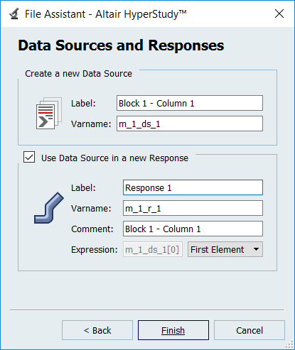
   Figure 4.

   Output response 1 is added to the work area.
8. Click Evaluate.
   The value for expression m_1_ds_1[0] should be 404.0.

1. Add an Optimization.
   1. In the Explorer, right-click and select Add from the context menu.
   2. In the Add dialog, select Optimization and click OK.
2. Go to the Optimization > Definition > Define Output Responses step.
3. Click the Objectives/Constraints - Goals tab.
4. Add an objective to Response 1.
   1. Click Add Goal.
   2. In the Type column, select Minimize.

   
   
   Figure 5.

5. Go to the Optimization > Specifications step.
6. In the work area, set the Mode to Adaptive Response Surface Method (ARSM).
   Note: Only the methods that are valid for the problem formulation are enabled.
7. Click Apply.
8. Go to the Evaluate step.
9. Click Evaluate Tasks.
10. Optional: Click the Iteration Plot tab to monitor the progress of the optimization.
    The iteration history shows a significant reduction in the objective value. The Rosenbrock function has a global minimum that is difficult for any optimizer to find due to its flatness in the area of the true optimum, and ARSM has not found the theoretical solution at (x,y)=(1,1).

    
    
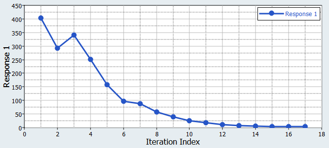
    Figure 6.