HS-1550: Shape Optimization Study Using HyperMesh and
Abaqus
Learn how to perform a shape optimization using HyperMesh
and HyperStudy. You will be using the finite element solver Abaqus, and HyperMorph to do the shape
parameterization. This tutorial also demonstrates how to solve a problem when HyperMesh and HyperStudy are running in Windows and
the solver is on a UNIX platform.
Before you begin, copy the model files used in
this tutorial from <hst.zip>/HS-1550/ to your working
directory.
In this tutorial, you will:
Use HyperMorph to generate a shape variable.
Run a study from inside HyperMesh.
Perform a shape parameterization using HyperStudy.
Set up a study.
Write a script to run Abaqus on UNIX and
register the script in the preference file.
Run an optimization study.
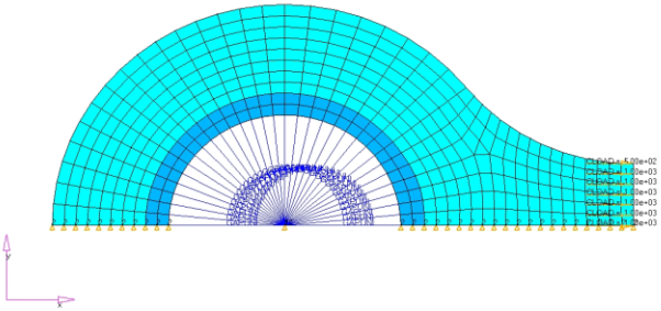
The objective of this tutorial is to minimize the mass of a link that is
connected to a shaft, given a stress constraint of 200MPa. The input variables are
defined by the outer shape. Figure 1.
Load the Model in HyperMesh
Start HyperMesh Desktop.
In the User Profiles dialog, set the user profile to
Abaqus, Standard2D.
From the menu bar, click File > Open > Model.
In the Open Model dialog, open the
link.hm file.
A finite element model appears in the graphics area. Figure 2.
Perform Shape Parameterization in HyperMorph
From the Tool page, click HyperMorph.
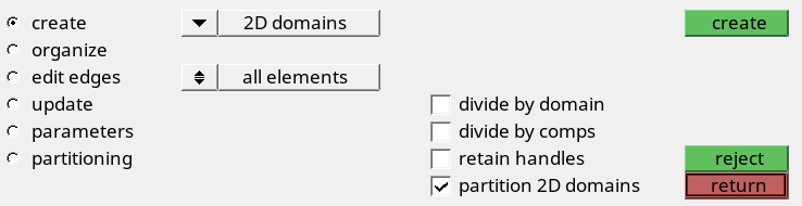
Create domains.
Click domains.
The Domains subpanel opens, from which you can create domains
for the shape parameterization.
Click the first arrow and select 2D
domains.
Click the toggle and select all elements.
Click create.
Figure 3.
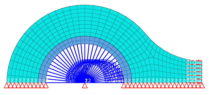
Domains and handles are generated and will be used to manipulate the
shape of the mesh and to generate shape perturbations required for the shape
optimization. Figure 4.
Click return.
Create an input variable for the outer edge of the link.
From the HyperMorph panel, click morph.
The Morph subpanel opens, from which you can morph the shape of
the mesh.
Click the second switch and select
translate.
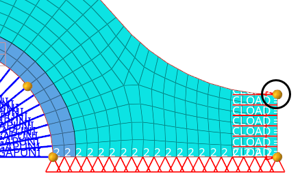
In the y val= field, enter -5.0.
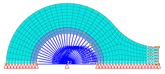
In the graphics area, click the yellow handle located at the top-right
corner of the link.
Figure 5.
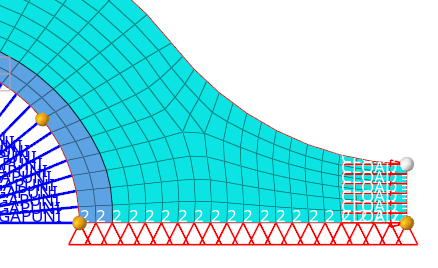
Click morph.
The first shape is generated. Figure 6.
Save the shape.
Go to the save shape subpanel.
In the name= field enter, sh1.
Click save.
Save the HyperMesh model by clicking File > Save > Model from the menu bar.
Close HyperMesh Desktop.
Set Up Basic Solver Script
In a text editor, open HS-1550_solverScript.py.
The HS-1550_solverScript.py files enables you to run the
solver on a local machine. This python script calls the Abaqus solver using
arguments that you specify.
Change the path in the file to the Abaqus executable on your machine.
Modify any additional arguments, such as memory requests.
# import statementsimport os
import platform
import subprocess
import sys
# user edits-------------------------------------------------------------------# set executable path use forward slashes (/)
exe_path = '/my/path/to/executable/abaqus.exe'# set abaqus arguments
command_arguments_list = ['job=' + sys.argv[1], 'memory=200Mb' , 'interactive']
# set log file name
logFile = 'logFile.txt'# -----------------------------------------------------------------------------# open log file
f = open('logFile.txt', 'w')
# get environment information
plat = platform.system()
hst_altair_home = ''
strEnvVal = os.getenv('HST_ALTAIR_HOME')
if strEnvVal:
hst_altair_home = strEnvVal
else:
f.write('%EXA_xx-e-env, Environment variable not defined ( HST_ALTAIR_HOME )')
exe_path = os.path.normpath(exe_path)
lstCommands = [exe_path] + command_arguments_list
# echo log information
f.write('platform: ' + plat + '\n')
f.write('hst_altair_home: ' + hst_altair_home + '\n')
f.write('command: ' + exe_path + '\n')
#Write the command in log file
f.write('Running the command:\n' + exe_path + ' ' + ' '.join(command_arguments_list) + '\n')
#Run the command
p1 = subprocess.Popen(lstCommands, stdout=subprocess.PIPE , stderr=subprocess.PIPE)
# log the standard out and error
f.write('\nStandard out' + '\n' + p1.communicate()[0] + '\n')
f.write('\nStandard error' + '\n' + p1.communicate()[1] + '\n')
# close log file
f.close()
Optional: Run HyperStudy on Windows with Study Directory in Unix and the Solver is
Running on Unix
Restriction: Only for remote machines.
In order to run
commands on a remote Unix machine, a local program must be installed to
communicate the commands remotely. In this example, the program ssh is being
used, but other equivalent or better programs exist. In most cases, the
program’s protocols require authentication from a password. For this setup
to work the environment needs to be configured to work without an active
password entry. This setup may require help from your network
administrators.
The ssh_remote.bat file is a sample (Windows) batch file
to run a script on Unix (run_abaqus.sh) from a
HyperStudy session running on
Windows.
The batch file uses the ssh command to log onto the Unix machine and execute
the solver on the files created by HyperStudy. This script will be
registered in HyperStudy as the solver script.
Open the ssh_remote.bat file
Change the generic parameter “unix_machine” to match
the name of the remote Unix machine on your network.
Change the generic parameter “user_name” to match your
logon on the remote machine.
Note: This logon should have been configured to work without a password
between these two machines.
Open the run_abaqus.sh file.
The run_abaqus.sh file is a shell script which is
designed to run the Abaqus solver on a UNIX machine. This file should be
placed in your HOME directory on the Unix
machine.
#!/bin/sh

#constuct the model directory
approachName=$1
runNum=`printf %05i $2`
modelString=$3
array=(${modelString//:/ })
modelName=${array[0]}
myDir=~/${approachName}/run__${runNum}/${modelName}

#change the directory to model directory
cd $myDir

#change the format from windows to unix
dos2unix $1 $1

#edit this line to match your solver path and the appropriate arguments
/my/path/to/solver/example/abaq631 job=$1 memory=200Mb interactive
Change the text formatting to be Unix compatible using the command
dos2unix on the file: dos2unix
run_abaqus.sh.
Make sure the file has executable permission, and enter
chmod 755 run_abaqus.sh.
Edit the run_abaqus.sh file and modify the path to
the executable and any other options to this command as needed.
Register Abaqus as a Solver
Start HyperStudy.
From the menu bar, click Edit > Register Solver Script.
The Register Solver Script dialog
opens.
Add solver script.
Click Add Solver Script.
The Add dialog opens.
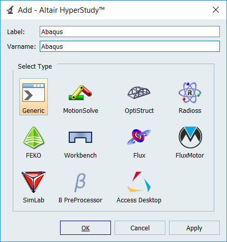
In the Label and Varname fields, enter
Abaqus.
From the list of solver script types, select
Generic.
Click OK.
Figure 7.
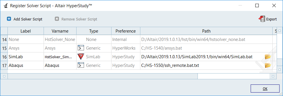
In the Path column of the script Abaqus, click .
In the Open dialog, open the
python.exe file.
Tip: You can also copy and paste the same path and file from the
Python Path field.
In the User Arguments column of the Abaqus script, click .
In the Open dialog, navigate to your working directory and
open the HS-1550_solverScript.py file.
Optional: ONLY for REMOTE Machines: Register Abaqus as a solver.
Figure 8.
Click OK.
Perform the Study Setup
Start a new study in the following ways:
From the menu bar, click File > New.
On the ribbon, click .
In the Add Study dialog, enter a study name, select a
location for the study, and click OK.
Note: The study directory MUST be your home on the mapped UNIX machine.
Go to the Define Models step.
Add a HyperMesh model.
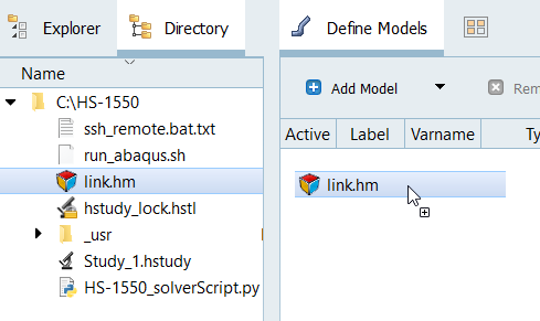
From the Directory, drag-and-drop the HyperMesh
(.hm) file link.hm into
the work area.
Figure 9.
In the Solver Input File column, enter
link.inp.
This is the name of the solver input file HyperStudy writes during any
evaluation.
In the Solver execution script column, select
Abaqus.
In the Solver Input Arguments column enter,
$filebasename.
Optional. In addition, you may need to edit the Abaqus environment
file (ex: <ABAQUS INSTALL>\v6.11\6.11-1\site\abaqus
v6.env) to include:
ask_delete=OFF
or
comment the line ask delete=on if any.
This is needed because Abaqus prompts you to overwrite the old files
when re-running the analysis. In order to eliminate the need for
user interaction, you need to command Abaqus not to ask this
question and overwrite.
Figure 10.
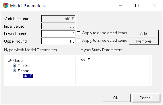
Import variables.
Click Import Variables.
The Model Parameters dialog
opens.
Expand Shape, and click
sh1.S.
Change the Lower bound to 0.0 and the Upper bound to 1.0.
Click Add.
Click OK.
Figure 11.
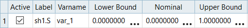
Go to the Define Input Variables step.
Review the design variable's lower bound, initial and upper bound range.
Figure 12.
Perform Nominal Run
Go to the Test Models step.
Click Run Definition.
An approaches/setup_1-def/ directory is created
inside the study Directory. The
approaches/setup_1-def/run__00001/m_1 directory
contains the input file, which is the result of the nominal run.
Create and Evaluate Output Responses
In this step you will create two output responses: Mass and Max_Stress.
Go to the Define Output Responses step.
Create the Mass output response.
From the Directory, drag-and-drop the link.dat
file, located in the
approaches/setup_1-def/run__00001/m_1
directory, into the work area.
In the File Assistant dialog, set the Reading
technology to Altair® HyperWorks® and click
Next.
Select Single item in a time series, then click
Next.
Define the following options, and then click
Next.
Set Type to ABAQUS.dat.
Set Request to TOTAL MASS.
Set Component to MASS.
Label the output response Mass.
Set Expression to First Element.
Click Finish.
The Mass output response is added to the work area.
Create the Max_Stress output response.
From the Directory, drag-and-drop the link.obd
file, located in the
approaches/setup_1-def/run__00001/m_1
directory, into the work area.
In the File Assistant dialog, set the Reading
technology to Altair® HyperWorks® and click
Next.
Select Multiple items at multiple time steps
(readsim), then click Next.
Define the following options, and then click
Next.
Set Subcase to Step-2.
Set Type to S-Global-Stress components
(PART-1-1).
Set Request to E1 -
E378.
Set Component to vonMises.
Label the output response Max_Stress.
Set Expression to Maximum.
Click Finish.
The Max_Stress output response is added to the work
area.
Click Evaluate to extract the response values.
Run Optimization
Add an Optimization.
In the Explorer, right-click and select
Add from the context menu.
In the Add dialog, select
Optimization and click OK.
Go to the Optimization > Definition > Define Output Responses step.
Click the Objectives/Constraints - Goals tab.
Add an objective.
Click Add Goal.
In the Apply On column, select Mass (r_1).
In the Type column, select Minimize.
Figure 13. Objective
Add a constraint.
Click Add Goal.
In the Apply On column, select Max_Stress (
r_2).
In the Type column, select Constraint.
In column 1, select <= (less than or equal
to).
In column 2, enter 200.0.
Figure 14. Constraint
Go to the Optimization > Specifications step.
In the work area, set the Mode to Adaptive
Response Surface Method (ARSM).
Note: Only the methods that are valid for the problem formulation are enabled.
Click Apply.
Go to the Optimization > Evaluate step.
Click Evaluate Tasks.
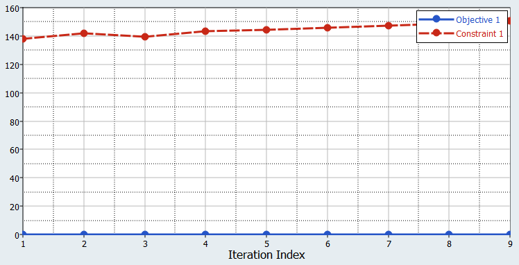
View the iteration history of the Optimization.
Click the Iteration History tab to review the
Optimization results.
The optimal design is highlighted in green.
Click the Iteration Plot tab to plot the
Optimization results.
 .
.
 .
.