Learn how to create various approaches (Design of Experiment, Approximation,
Optimization, Stochastic) and explore a variety of tools and post processing methods offered
by HyperStudy.
In the Explorer, right-click and select
Add from the context menu.
In the Add dialog, select
DOE and click OK.
Define specifications.
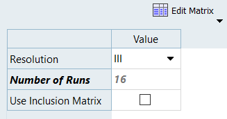
Go to the DOE 1 > Specifications step.
In the work area, set the Mode to Fractional
Factorial.
In the Settings tab, set Resolution to
III.
Figure 1.
Click Apply.
Evaluate tasks.
Go to the DOE 1 > Evaluate step.
Click Evaluate Tasks.
While the DOE is in progress, click the
Tasks tab to view the feedback on the results
of the evaluation.
During the execution of the DOE, you can
monitor the evaluation of the 16 runs in either the Evolution
Plot or Evolution Data
tabs.
Post process results.
Go to the DOE 1 > Post-Processing step.
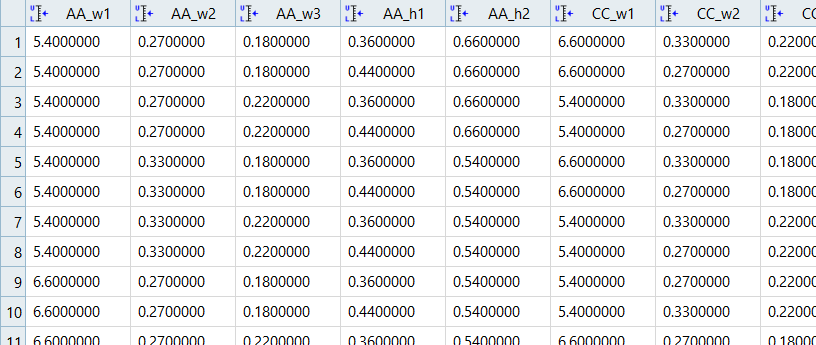
Click the Summary tab to view all input variable
and output response run data in a table.
Tip: Use the Sort and
Find options in the right-click context menu to sort and search data.
Figure 2.
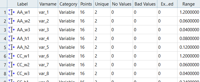
Click the Integrity tab to view statistical
measures over the population (samples of the DOE) for all of the input variables and output
responses.
Figure 3.
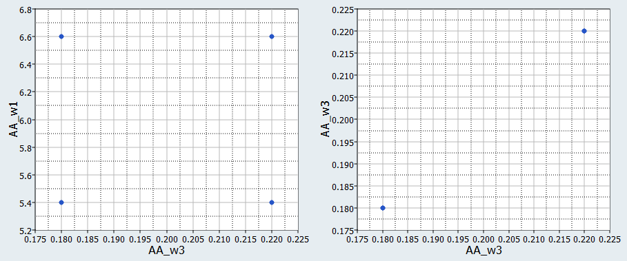
Click the Scatter tab to plot the DOE results.
Figure 4.
Click the 3D Scatter tab to view DOE results in a scatter plot.
Tip: If the 3D Scatter tab is not enabled, click (Show or
Hide Tabs), and select 3D Scatter from the
Standard Tabs.
Only one input variable/output response can be
selected for the X and Y axes, whereas multiple input variables/output
responses can be selected for the Z axis. Figure 5.
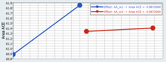
Click the Linear Effects tab to review the
effect of an input variable on an output response, ignoring the effects
of other input variables.
Above the Channel selector, click to plot the
linear effects. Use the Channel selector to select the variables
AA_w1 and AA_w2 and
the output response Area ACE.
Figure 6.
Above the Channel selector, click to view the
linear effects in a table.
Tip: From the Channel selector, use the
Sort and Filter
options in the right-click context menu to sort and filter
effects.
Figure 7.
Run Hammersley DOE
Add a DOE.
In the Explorer, right-click and select
Add from the context menu.
In the Add dialog, select
DOE and click OK.
Define specifications.
Go to the DOE 2 > Specifications step.
In the work area, set the Mode to
Hammersley.
In the Settings tab, change the Number of Runs
to 50.
Click Apply.
Evaluate tasks.
Go to the DOE 1 > Evaluate step.
Click Evaluate Tasks.
Run Latin HyperCube DOE
Add a DOE.
In the Explorer, right-click and select
Add from the context menu.
In the Add dialog, select
DOE and click OK.
Define specifications.
Go to the DOE 3 > Specifications step.
In the work area, set the Mode to Latin
HyperCube.
In the Settings tab, change the Number of Runs
to 15.
Click Apply.
Evaluate tasks.
Go to the DOE 1 > Evaluate step.
Click Evaluate Tasks.
Run Radial Basic Function Fit
Add a Fit.
In the Explorer, right-click and select
Add from the context menu.
In the Add dialog, select
Fit and click OK.
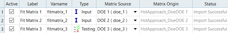
Import matrices
Go to the Fit 1 > Specifications step.
Click Add Matrix three times to add three
matrices.
Define the matrices by selecting the options indicated in the Figure 8.
Click Apply.
Figure 8.
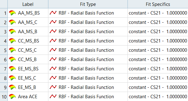
Define specifications.
In the work area, Fit Type column, select Radial Basis
Function (RBF) for all output responses.
Click Apply.
Figure 9.
Evaluate Fit.
Go to the Fit 1 > Evaluate step.
Click Evaluate Tasks.
To review the values of the output responses and their approximations
while the evaluation is in progress, click the Evaluation
Data and Evaluation Plot
tabs.
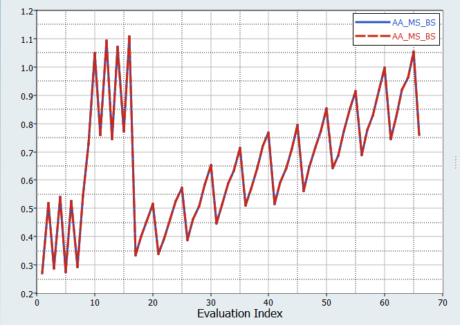
Figure 10. Evaluation Plot
Post process results.
Go to the Fit 1 > Post-Processing step.
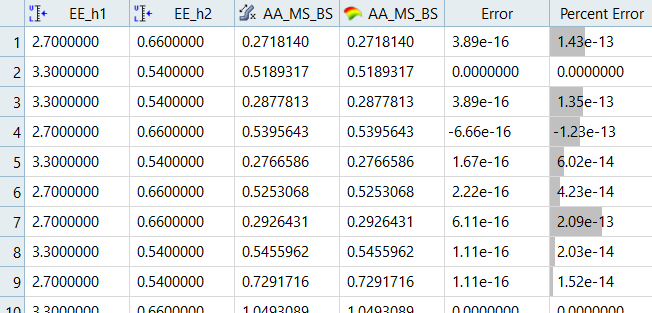
Click the Residuals tab to identify errors for
each design.
The error (and percentage) between the original output response and
the approximation is listed for each run of the input,
cross-validation, or testing matrices. Figure 11.
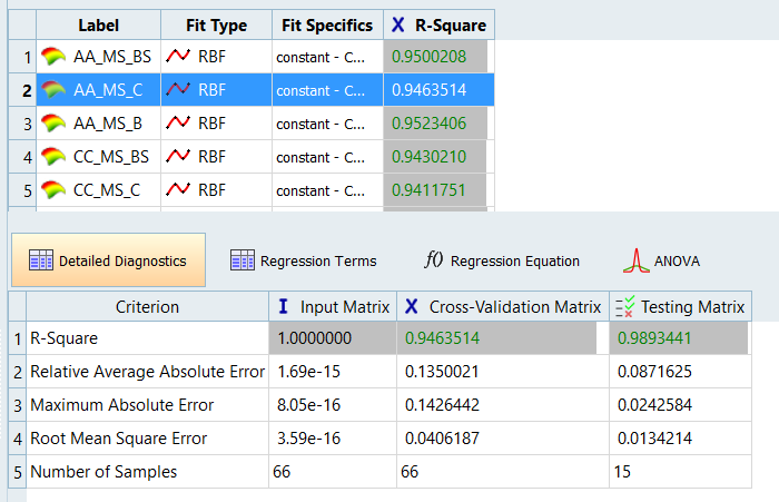
Click the Diagnostics tab to assess the accuracy
of a Fit. Different criteria is displayed for the Input, Testing, and
merged matrices.
Figure 12.
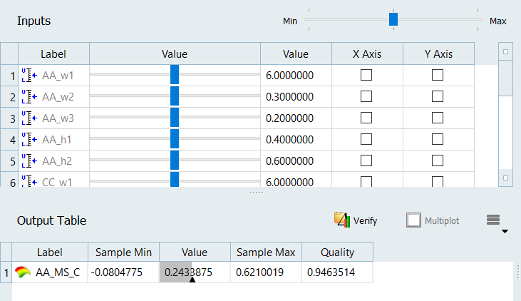
Click the Trade-Off tab to modify the values of
input variables in order to see their effect on the output response
approximations.
Use the Channel selector to select the desired
output responses to display in the Outputs pane. Input variable controls
are located in the top frame (Inputs). Change each input variable by
moving the slider in the first Value column, or
by entering a value into the second Value column.
Set input variables to their initial, minimum, or maximum values by
moving the slider in the upper right-hand corner of the Inputs
frame. Figure 13.
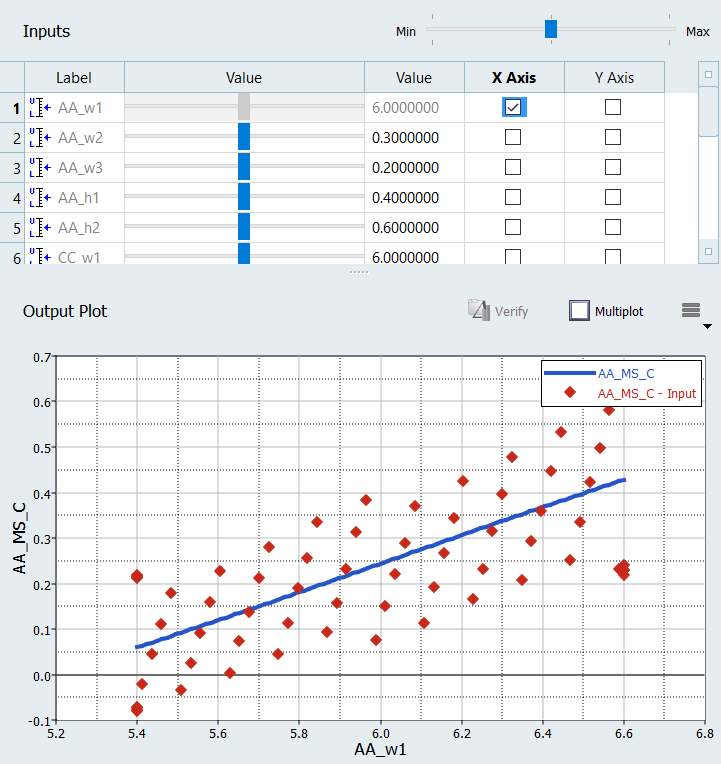
In the Trade-Off tab plot variables and output
responses in order to see the input variables effect on the output
response approximations.
Select input variables to plot by enabling its corresponding
X Axis checkbox in the Inputs pane. Use the
Channel selector to select output responses
to plot. The values for the input variables which are not plotted are
modified in the top frame (Inputs). Move the sliders in the
Value column to modify the other input
variables, while studying the output response throughout the design
space. Figure 14.
Run ARSM Optimization
Add an Optimization.
In the Explorer, right-click and select
Add from the context menu.
In the Add dialog, select
Optimization and click OK.
Go to the Optimization 2 > Definition > Define Output Responses step.
Click the Objectives/Constraints - Goals tab.
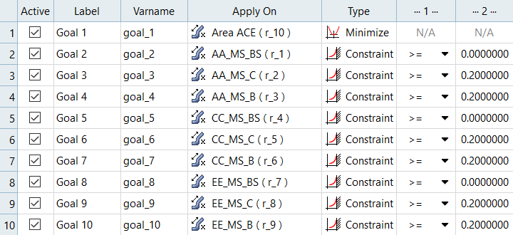
Add an objective.
Click Add Goal.
In the Apply On column, select Area ACE
(r_10).
In the Type column, select Minimize.
Figure 15.
Add constraints.
Click Add Goal nine times to add nines goals,
which will be defined as constraints.
Define Constraint 1 through Constraint 9 by selecting the options
indicated in Figure 16.
Figure 16.
Define specifications.
Go to the Optimization 2 > Specifications step.
In the work area, set the Mode to Adaptive Response Surface
Method (ARSM).
Note: Only the methods that are valid for the problem formulation are
enabled.
Click Apply.
Evaluate tasks.
Go to the Optimization 2 > Evaluate step.
Click Evaluate Tasks.
Click the different tabs in the Evaluate step to
monitor the progress of the Optimization.
Click the Evaluation Plot tab to plot variables
and output responses across runs (abscissa are run numbers, not
iterations).
Figure 17.
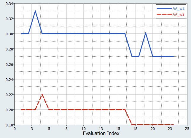
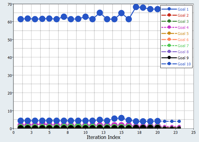
Click the Iteration Plot tab to plot variables
and output responses against iterations.
Figure 18.
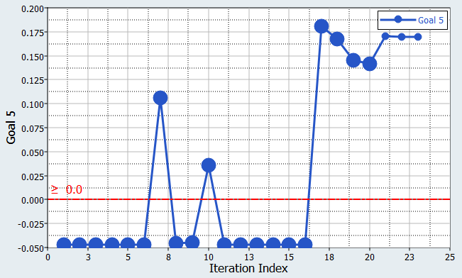
When the constraint history is plotted, the constraint bounds can
be marked with a datum line. Use the Channel selector to select a
constraint, then click (located above the
Channel selector) and select Bounds. Figure 19.
Run Hammersley Stochastic
Add a Stochastic.
In the Explorer, right-click and select
Add from the context menu.
In the Add dialog, select
Stochastic and click OK.
Define specifications.
Go to the Stochastic > Specifications step.
In the work area, set the Mode to
Hammersley.
In the Settings tab, change the Number of Runs
to 100.
Click Apply.
Evaluate tasks.
Go to the Stochastic > Evaluate step.
Click Evaluate Tasks.
Go to the Stochastic > Post-Processing step.
Click the Integrity tab to access a series of
statistical measures on input variables and output responses.
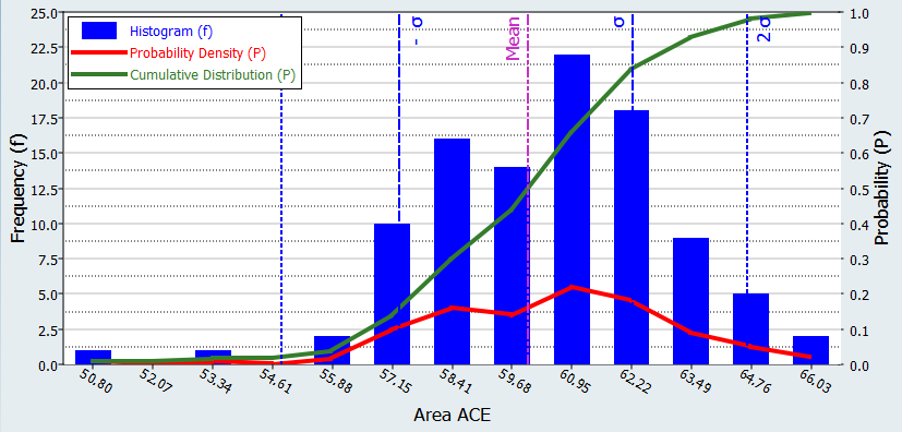
Click the Distribution tab to view variable and output
response data in a histogram.
Figure 20.
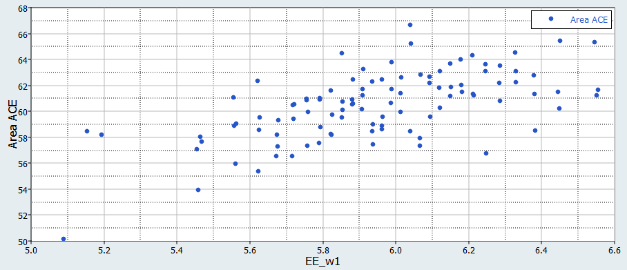
Click the Scatter tab to view sampling patterns and
possible correlations between output responses or between input variables and
output responses.
Figure 21.
Compute the probability of failure (bound is violated) and the reliability
(bound is respected).
Click the Reliability tab.
Click Add Reliability.
Define the reliability.
Set Response to Area ACE (r_10).
Set Bound Type to <= (less than or
equal to).
For Bound Value, enter 70.000.
HyperStudy computes the reliability and probability of failure
in the Reliability and Probability of Failure columns. Figure 22.
 (Show or
Hide Tabs), and select 3D Scatter from the
Standard Tabs.
(Show or
Hide Tabs), and select 3D Scatter from the
Standard Tabs.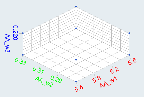
 to plot the
linear effects. Use the Channel selector to select the variables
AA_w1 and AA_w2 and
the output response Area ACE.
to plot the
linear effects. Use the Channel selector to select the variables
AA_w1 and AA_w2 and
the output response Area ACE.
 to view the
linear effects in a table.
Tip: From the Channel selector, use the Sort and Filter options in the right-click context menu to sort and filter effects.
to view the
linear effects in a table.
Tip: From the Channel selector, use the Sort and Filter options in the right-click context menu to sort and filter effects.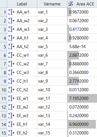

 (located above the
Channel selector) and select Bounds.
(located above the
Channel selector) and select Bounds.