HS-2215: Extensible DOE Study of a Space Frame Structure with Input Variable Constraints
Learn how to use a DOE to investigate the effects of the cross sectional dimensions and joint stiffness of a truss structure’s volume and natural frequencies.
The tubular truss dimensions must be constrained, such that the inner radius is always less than the outer radius. You will also use the extensible feature of the Modified Extensible Lattice Sequence in a progressive set of steps to add additional runs to a DOE.
Perform the Study Setup
-
Start a new study in the following ways:
- From the menu bar, click .
- On the ribbon, click
 .
.
-
Add a Parameterized File model.
-
From the Directory, drag-and-drop the
tinker_toy.tpl file into the work area.
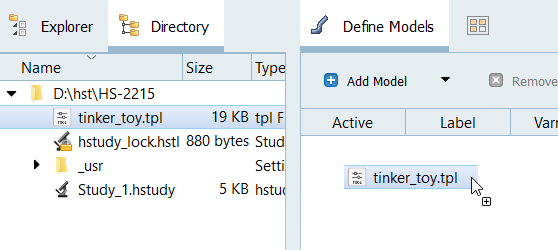
Figure 1. -
In the Solver input arguments column, after ${file}, enter
-core in.
This option forces OptiStruct to run with maximum memory, which will make the analysis run more quickly. The small size of the finite element model makes this possible in this example.
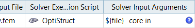
Figure 2.
-
From the Directory, drag-and-drop the
tinker_toy.tpl file into the work area.
-
Add an input variable constraint.
-
Use the Expression Builder to select input
variables to append to the Left Expression and Right Expression
fields.
- For Left Expression, select outer_diam.
- Set Comparison to >=.
- For Right Expression, select inner_diam.

Figure 3.
-
Use the Expression Builder to select input
variables to append to the Left Expression and Right Expression
fields.
Perform Nominal Run
Create and Define Output Responses
-
Create the Volume output response.
-
Define the following options, and then click
Next.
- Set Type to Volume.
- Set Request to Volume.
- Set Component to Value.
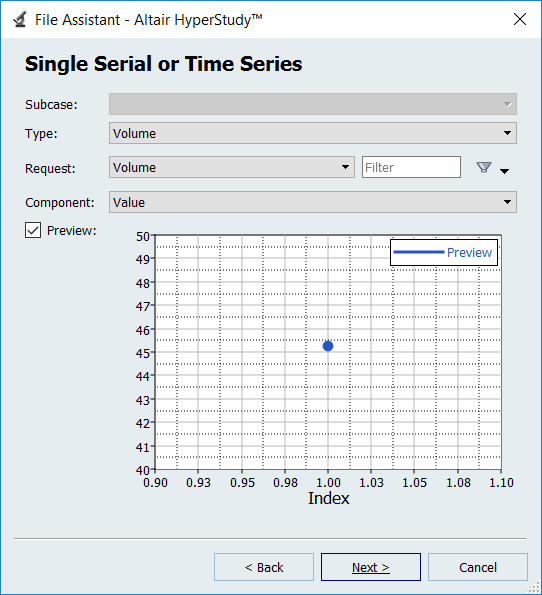
Figure 4. -
Click Finish.
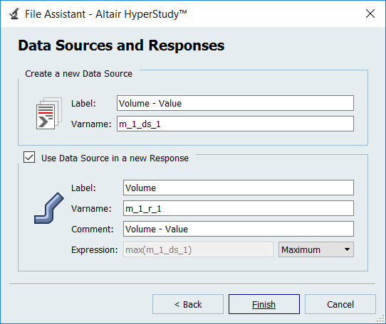
Figure 5.
-
Define the following options, and then click
Next.
-
Create the Frequency_Vector data source, which will be used in the frequency
output responses.
-
Click OK.
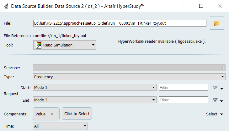
Figure 6. -
In the work area, Label column, change the label for Data Source 2 to
Frequency_Vector.
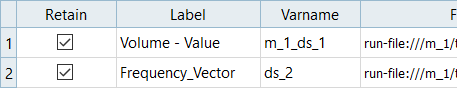
Figure 7.
-
Click OK.
-
Add three output responses.
- Click the Define Output Responses tab.
- Click Add Output Response three times.
- In the work area, label the output responses Frequency_1, Frequency_2, and Frequency_3.
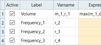
Figure 8. -
Define the Frequency_1 output responses.
-
From the Insert Varname drop-down menu, click First
Element.
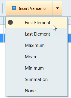
Figure 9. -
Click Insert Varname.
The expression ds_2[0] appears in the Evaluate Expression field.
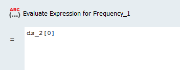
Figure 10.
-
From the Insert Varname drop-down menu, click First
Element.
-
Repeat step 5 to define Frequency_2 and Frequency_3, except change the
value after ds_2.
- For Frequency_2, change [0] to [1].
- For Frequency_3, change [0] to [2].
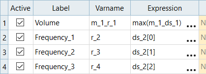
Figure 11.
Run MELS DOE Study, with Four Runs
-
In the Settings tab, change the Number of Runs to
4.
This is the minimum number of runs for a multivariate effects calculation.
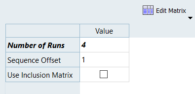
Figure 12. -
Click the Scatter tab, and using the Channel selector to
set the X Axis to Outer_diameter and the Y Axis to
Inner_diameter.
All four runs satisfy the constraint, which is inner_radius < outer_radius.
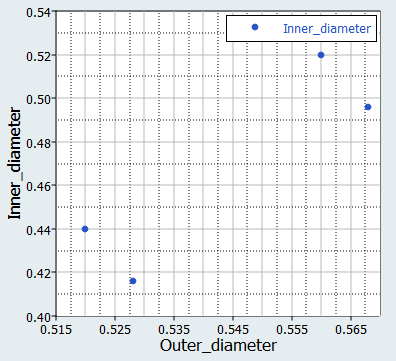
Figure 13. -
Review Pareto plot.
- Click the Pareto Plot tab.
- Above the Channel selector, click and verify that Multivariate effects is selected.
- Note which input variables contribute to which output responses.
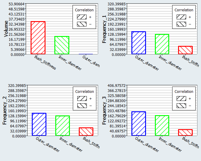
Figure 14.
Extend DOE with Seven Additional Runs
In this step you will run a second Modified Extensible Lattice Sequence DOE study with seven new runs, and include the four runs from DOE1.
This DOE will have a total of 11 runs, which is the default suggested number of runs for a MELS DOE with three input variables.
-
Import run data from the DOE 1 using an Inclusion Matrix.
-
Click from the top, right corner of the work area.
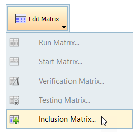
Figure 15.
-
Click from the top, right corner of the work area.
-
Click the Scatter tab, and use the Channel selector to
set the X Axis to Outer_diameter and the Y Axis to
Inner_diameter.
All 11 runs still satisfy the constraint, which is inner_radius < outer_radius.
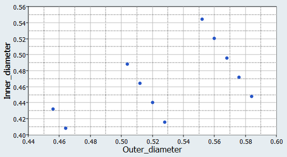
Figure 16. -
Click the Pareto Plot tab, and compare the results to
the Pareto Plot from DOE 1.
The magnitude and order of importance has changed in some cases.
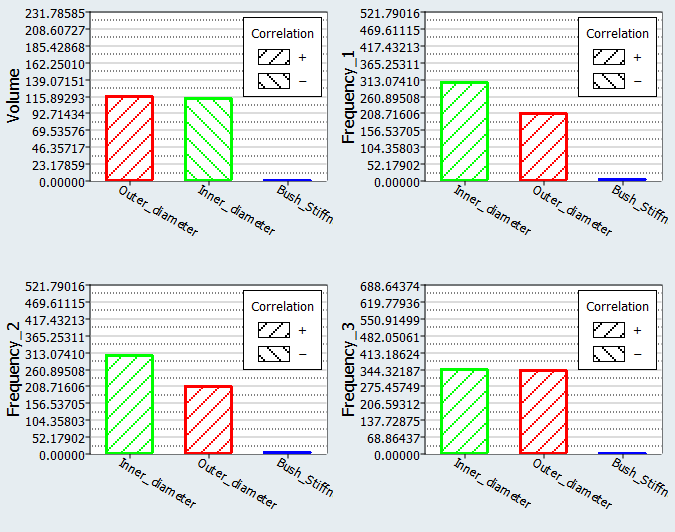
Figure 17. Pareto Plot from DOE 2
Figure 18. Pareto Plot from DOE 1
Extend DOE with Four Additional Runs
In this step you will run a third Modified Extensible Lattice Sequence DOE study with four new runs, and include the 11 runs from DOE 2.
-
Click the Pareto Plot tab, and compare the results to
the Pareto Plots from DOE 2.
The results are qualitatively the same, indicating that you will likely have enough runs to draw solid conclusions.
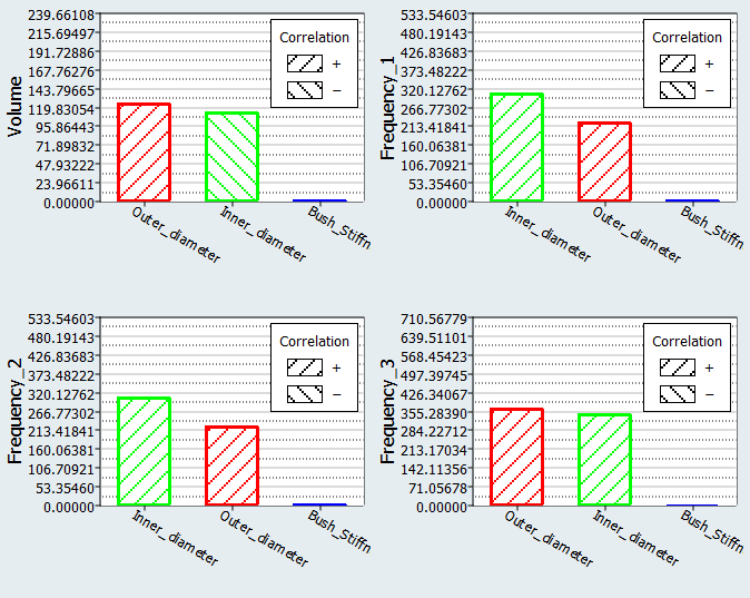
Figure 19. Pareto Plot from DOE 3
Figure 20. Pareto Plot from DOE 2