HS-4000: Optimization Method Comparison: Arm Model Shape Optimization
Learn how to perform an Optimization and compare different methods for efficiency and effectiveness.
- Volume = 1.77E+06 mm3
- Max_Disp = 1.41 mm
- Max_Stress = 195.29 MPa
In this tutorial, the Optimization objective is to reduce Volume, while respecting a constraint on Max_Disp that should be less than 1.5 mm.
In HS-3000: Fit Method Comparison - Approximation on the Arm Model, you learned that it was difficult to accurately capture the Max_Stress function using a Fit approximation. In the DOE analysis, you learned that most of the tested design configurations for Max_Stress were below 300 MPa. For these reasons, you will not consider a constraint on the Max_Stress function. Max_Stress values can be collected throughout the Optimization when running the exact solver.
ARSM, Six Input Variables, Exact Solver
-
In the Active column of the work area, clear the
radius_1, radius_2 and
radius_3 checkboxes.
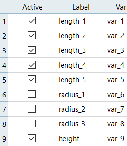
Figure 1. -
Add an objective.
- Click Add Goal.
- In the Apply On column, select Volume.
- In the Type column, select Minimize.

Figure 2. -
Add a constraint.
- Click Add Goal.
- In the Apply On column, select Max_Disp.
- In the Type column, select Constraint.
- In column 1, select <= (less than or equal to).
- In column 2, enter 1.5.
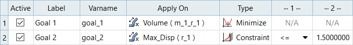
Figure 3. -
Click the Iteration History tab to view the optimum
solution, which is highlighted green in the table.
Note: The optimal design for Max_Stress is equal to 215, which is lower than 300.
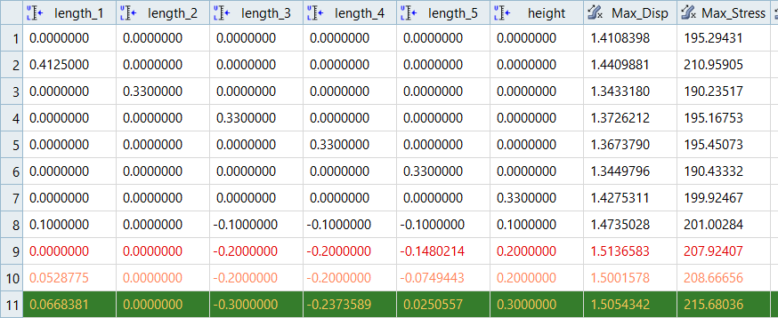
Figure 4. -
Click the Iteration Plot tab to review the results of
the optimization in an iteration plot.
-
Select the Objective (Volume) and
Constraint (Max_Disp) functions to see their
variations during the Optimization process.
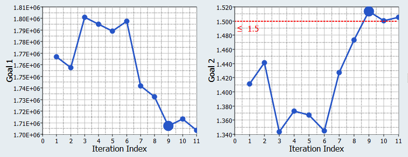
Figure 5. -
Select all of the design variables to see their variations during the
Optimization process.
Note: Check if any of the input variables meet their bounds in the optimal design. If any input variable's values meet their bounds, this indicates that relaxing these bounds may enable you to find better solutions. In Figure 6, only length_2 and length_5 meet their lower bounds.
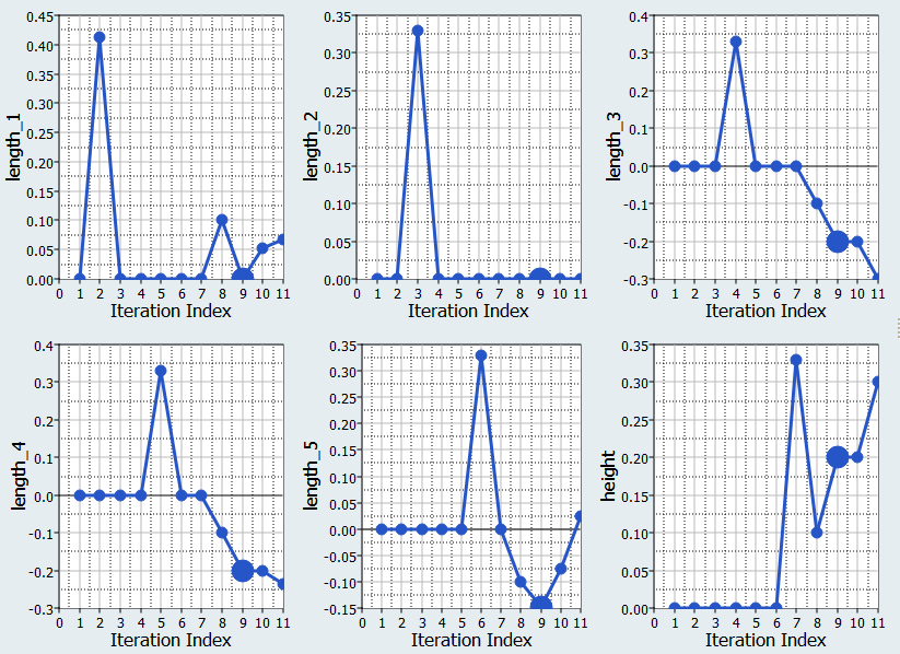
Figure 6.
-
Select the Objective (Volume) and
Constraint (Max_Disp) functions to see their
variations during the Optimization process.
ARSM, Nine Input Variables, Exact Solver
-
Select the Objective (Volume) and
Constraint (Max_Disp) functions to see their
variations during the Optimization process.
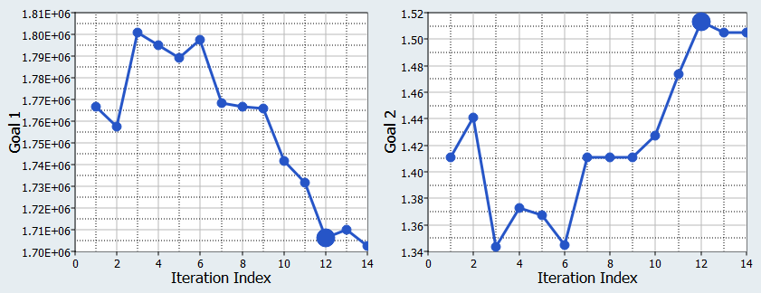
Figure 7.
GRSM, Six Input Variables, Exact Solver
-
Click the Iteration history tab to review the results of
the Optimization in a table.
Note: The optimal solution is found at the 19th evaluation (from 50).
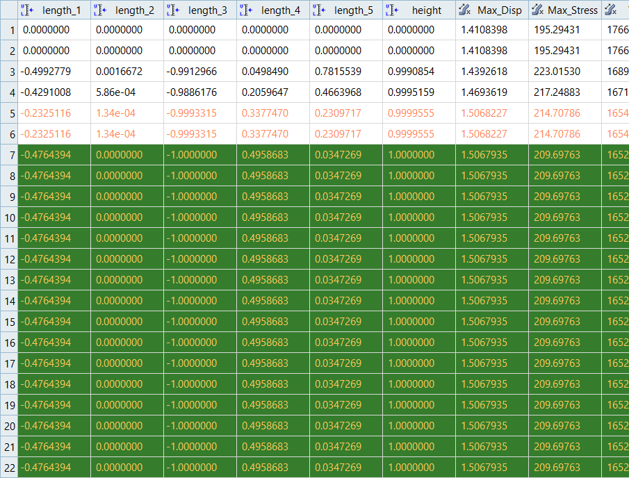
Figure 8. -
Review the results of the Optimization in an iteration plot.
-
Select the Objective (Volume) and
Constraint (Max_Disp) functions to see their
variations during the Optimization process.
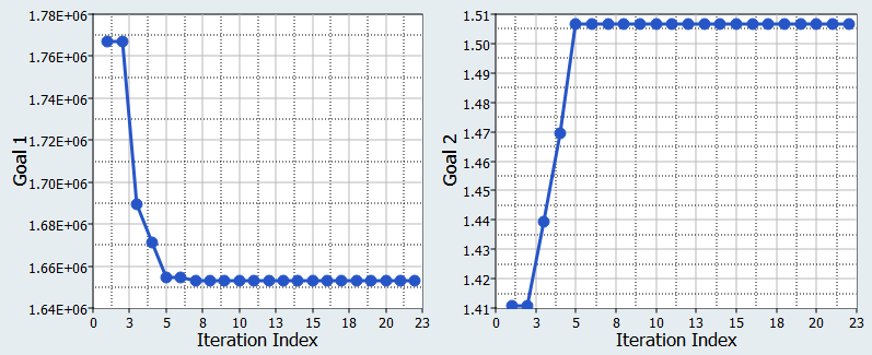
Figure 9.
-
Select the Objective (Volume) and
Constraint (Max_Disp) functions to see their
variations during the Optimization process.
SQP, Six Input Variables, Exact Solver
-
Select the Objective (Volume) and
Constraint (Max_Disp) functions to see their
variations during the Optimization process.
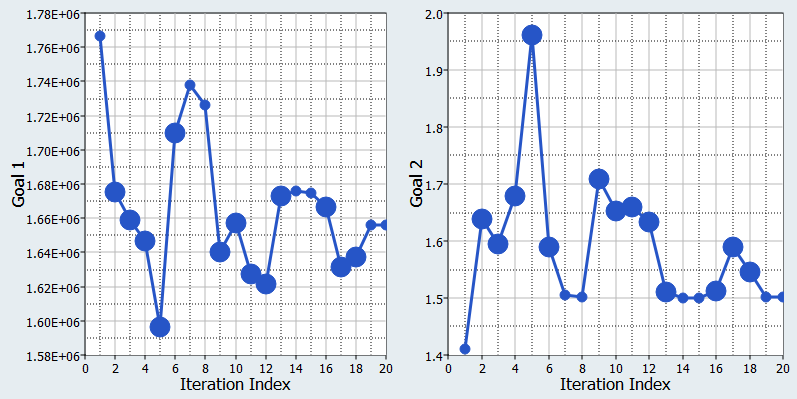
Figure 10.
SQP, Six Input Variables, RBF_MELS
-
Run a single objective, deterministic Optimization study by repeating ARSM, Six Input Variables, Exact Solver, except
change the following:
- Go to step, set Evaluate From to Fit, RBF (fit_4) for Max_Disp and Volume.
- In the Active column, clear the checkbox for Max_Stress.
- In the step, set the Mode to Sequential Quadratic Programming (SQP).
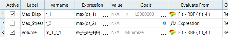
Figure 11. -
Review the results of the Optimization in an iteration plot.
- Click the Iteration Plot tab.
- Select the Objective (Volume) and Constraint (Max_Disp) functions to see their variations during the Optimization process.
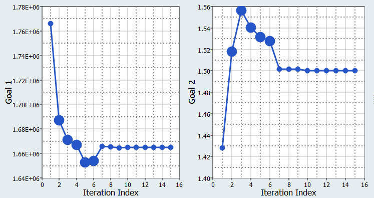
Figure 12. -
For Optimizations using a Fit, it is recommended that you perform a validation
run of the optimal solution.
-
Select the parameter values for the optimal solution, then right-click
and select Copy (Ctrl + C) from the context menu.
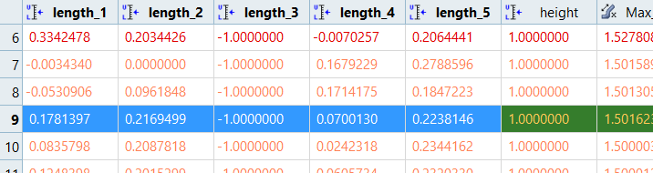
Figure 13. -
Click from the top-right corner of the work area.
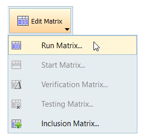
Figure 14.The Edit Run Matrix dialog opens. -
For height, enter 1.
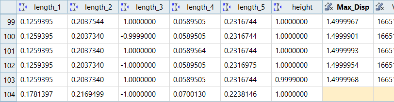
Figure 15. -
Click the Evaluate Data tab and compare the
Volume and Max_Disp values to those found by the Optimization.
Notice the similarity.
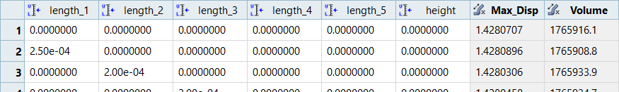
Figure 16.
-
Select the parameter values for the optimal solution, then right-click
and select Copy (Ctrl + C) from the context menu.
GA, Six Input Variables, RBF_MELS
-
Review the results of the Optimization in an iteration plot.
- Click the Iteration Plot tab.
- Select the Objective (Volume) and Constraint (Max_Disp) functions to see their variations during the Optimization process.
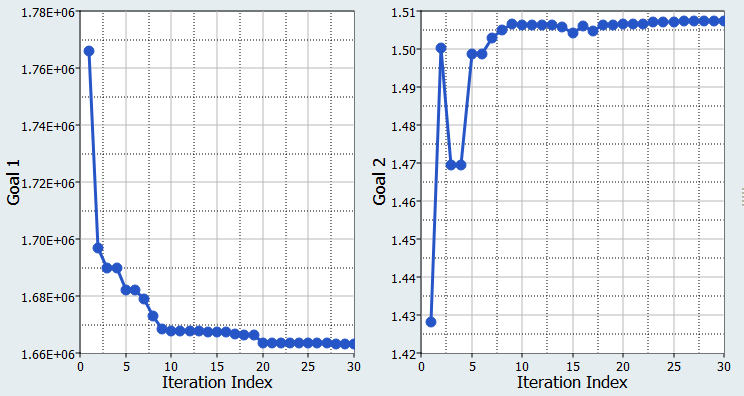
Figure 17.
Optimization Methods Comparison
| Optimization Method | # of Evaluations | Volume Objective |
|---|---|---|
| ARSM, 9 IVs, Exact Solver | 14 | 1702450.0 |
| ARSM, 6 IVs, Exact Solver | 11 | 1703330.0 |
| GRSM, 6 IVs, Exact Solver | 50 (22nd is the optimum) | 1652830.0 |
| SQP, 6 IVs, Exact Solver | 179 | 1659730.0 |
| SQP, 6 IVs, Fit | - | 1666990.6 |
| GA, 6 IVs, Fit | - | 1665387.3 |
Reliability-Based Design Optimization Study
In this step, run a reliability based design optimization study.
This topic will be discussed in HS-5000: Stochastic Method Comparison: Stochastic Study of the Arm Model
Multi-Objective Optimization Study
In this step, you will run a multi-objective optimization study.
This topic will be discussed in HS-4425: Multi-Objective Shape Optimization Study.