HS-4200: Material Calibration Using System Identification
Learn a method for characterizing parameters of a RADIOSS material law used for modeling elasto-plastic material.
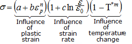
The characterization of a ductile aluminum alloy is studied. A RADIOSS simulation is performed to replicate an experimental tensile test. The parameters of the material law are determined to fit the experimental results.
HS-1506: Material Calibration with a Curve Difference Integral provides an alternative method to setup this problem using a HyperMath or Python function to measure the difference between two curves.
HS-1507: Material Calibration with Area Tool in Data Source provides an alternative method to set up this problem using the Area tool.
Model Definition
A quarter of a standard tensile test specimen is modeled using symmetry conditions. A traction is applied to a specimen via an imposed velocity at the left-end.
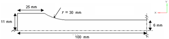
Figure 1. Geometry of the Tensile Specimen (One Quarter of the Specimen is Modeled)
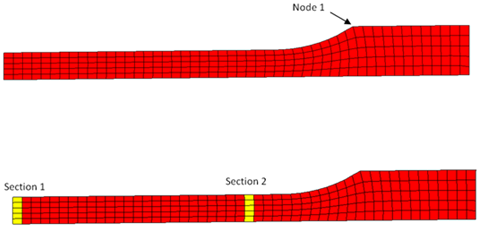
Figure 2. Sections of Node Saved for Time History
- Stress level
- Plastic strain
- Yield Stress
- Hardening modulus
- Hardening exponent
- Strain rate coefficient
- Strain rate
- Reference strain rate
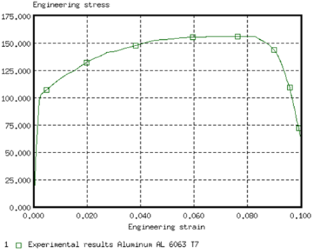
Figure 3. Engineering Stress Versus Engineering Strain Curve (Experimental Data)
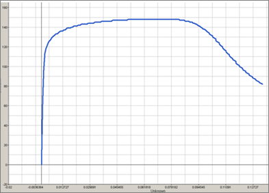
Figure 4. Engineering Stress Versus Strain Curve (Simulation Results)
Create Base Input Template
In this step, create the base input template in HyperStudy or use the base input template in the study directory.
-
In the Find area, enter /MAT/PLAS_JOHNS/1 and click
 .
HyperStudy highlights /MAT/PLAS_JOHNS/1 in the TENSILE_TEST_0000.rad file.
.
HyperStudy highlights /MAT/PLAS_JOHNS/1 in the TENSILE_TEST_0000.rad file.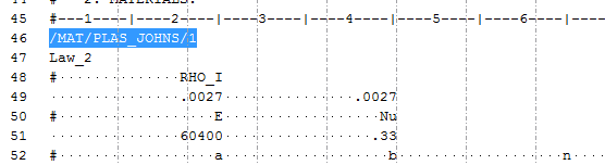
Figure 5. -
Select E by starting at the beginning of row 51 and
highlighting the first 20 fields.
Tip: To assist you in selecting 20-character fields, press Control to activate the Selector (set to 20 characters) and then click the value.
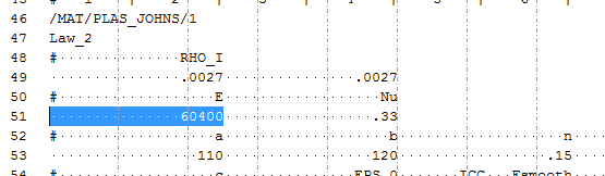
Figure 6. -
Click OK.
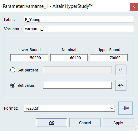
Figure 7.
Perform the Study Setup
-
Start a new study in the following ways:
- From the menu bar, click .
- On the ribbon, click
 .
.
-
Add a Parameterized File model.
-
From the Directory, drag-and-drop the
TENSILE_TEST_0000.tpl file into the work
area.
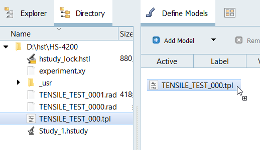
Figure 8.
-
From the Directory, drag-and-drop the
TENSILE_TEST_0000.tpl file into the work
area.
-
Define a model dependency
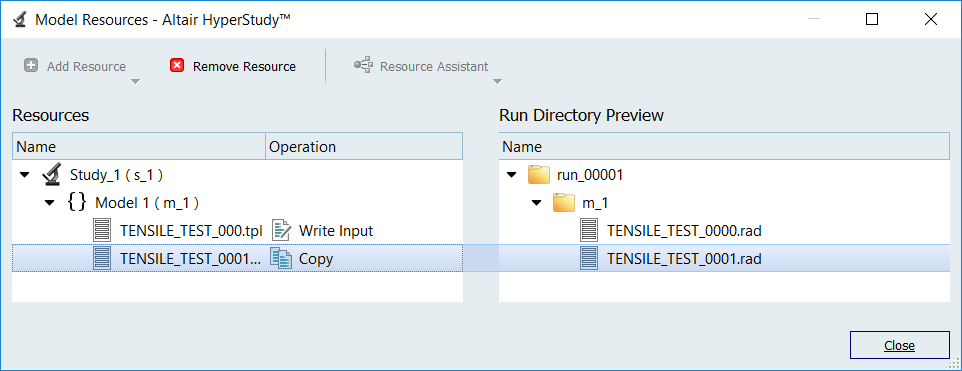
Figure 9.
Perform Nominal Run
Create and Evaluate Output Responses
In this step, you will compare RADIOSS stress-strain curve to the experimental data.
- Difference between experimental stress and RADIOSS at Strain equal 0.02 (1)
- Difference between experimental strain and RADIOSS at Necking point (2)
- Difference between experimental stress and RADIOSS at Necking point (3)
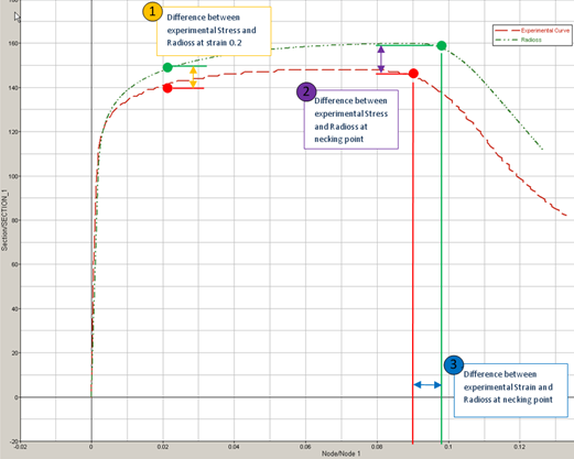
Figure 10.
- Go to the Define Output Responses step.
-
Create a data source labeled Disp_sim.
-
Click OK.
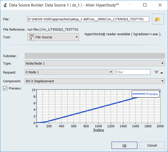
Figure 11. -
In the work area, change the label for the data source to
Disp_sim.
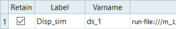
Figure 12.
-
Click OK.
-
Repeat step 2 to
create a second data source labeled Force_sim, making the
following changes during the process:
- Set Type to Section/SECTION_2.
- Set Request to 2 section 1.
- Set Component to FT-Resultant Tangent Force.
-
Create three output responses.
-
In the work area, Label column, change the labels for the three output
responses to Radioss_Strain_0_2,
Radioss_Stress_Necking, and
Radioss_Strain_Necking.
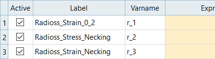
Figure 13.
-
In the work area, Label column, change the labels for the three output
responses to Radioss_Strain_0_2,
Radioss_Stress_Necking, and
Radioss_Strain_Necking.
-
Define the Radioss_Strain_0_2 output response.
-
In the Evaluate Expression field, enter
(ds_1/75,ds_2/10.2,0.02) in the lininterp
function.
This expression computes the Stress with respect to the Strain, at Strain equals 0.02.
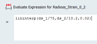
Figure 14.
-
In the Evaluate Expression field, enter
(ds_1/75,ds_2/10.2,0.02) in the lininterp
function.
-
Define the Radioss_Stress_Necking output response.
-
From the Insert Varname drop-down, select
Maximum.
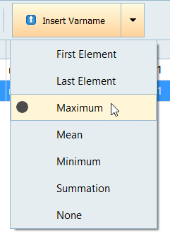
Figure 15.
-
From the Insert Varname drop-down, select
Maximum.
-
Define the Radioss_Strain_Necking output response.
- Click Evaluate to extract the response values.
Run Optimization
-
Review iteration history.
-
Activate
 to see the
each channel in its own plot.
to see the
each channel in its own plot.
-
Using the Channel selector, select the three objectives and Objective
Function.
The first three selections are the actual values used in the system identification optimization problem. Observe their objective history to see that their values indeed approach their respective target values. The final plot is the scalar objective which is used in the system identification problem; a normalized sum of the squares difference between the actual and target objective values. Note that the value of this combined function has been reduced through the optimization.
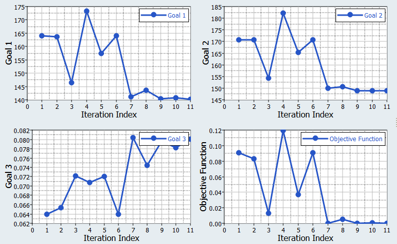
Figure 17.
-
Activate