HS-4230: Optimization Study with Discrete Variables
Learn how to use discrete variables.
The objective of this tutorial is to maximize the minimum frequency of the first five modes of a plate. The input variables are the thickness of each of the three components, defined in the input deck via the PSHELL card. The thickness should be between 0.05 and 0.15; the initial thickness within the files is 0.1. The optimization type is size. Furthermore, optimum design should have input variables from a discrete set of 0.05, 0.08, 0.11, and 0.14 for all three thicknesses. By default, HyperStudy will add the values from the lower and upper bounds to this set. Hence the resulting set is 0.05, 0.08, 0.11, 0.14, and 0.15. Delete any of these values if needed.
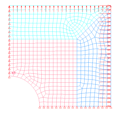
Figure 1. Double Symmetric Plate Model
Perform the Study Setup
-
Start a new study in the following ways:
- From the menu bar, click .
- On the ribbon, click
 .
.
-
Add a Parameterized File model.
-
From the Directory, drag-and-drop the plate.tpl
file into the work area.
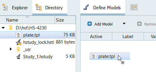
Figure 2.
-
From the Directory, drag-and-drop the plate.tpl
file into the work area.
-
Change Property 21 to be discrete.
-
In the Modes column of Property 21, select
Discrete.
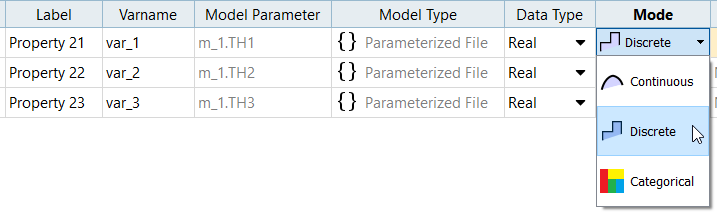
Figure 3. -
Click Step Size, enter
0.03, and click
Set.
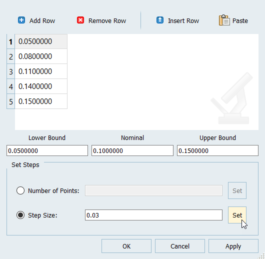
Figure 4.
-
In the Modes column of Property 21, select
Discrete.
Perform Nominal Run
Create and Evaluate Output Responses
In this step you will create two output responses.
- Go to the Define Output Responses step.
-
Create the Freq1 output response.
-
Define the following options and click
Next.
- Set Type to Frequency.
- Set Request to Mode 1.
- Set Component to Value.
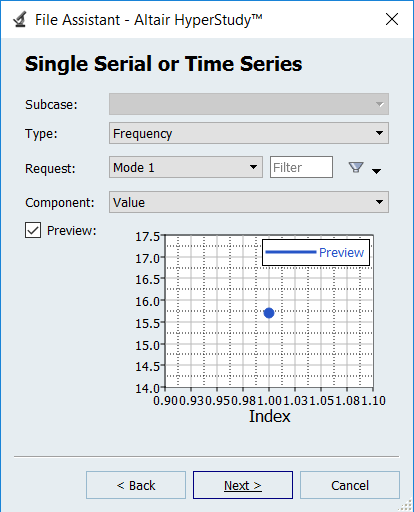
Figure 5. -
Click Finish.
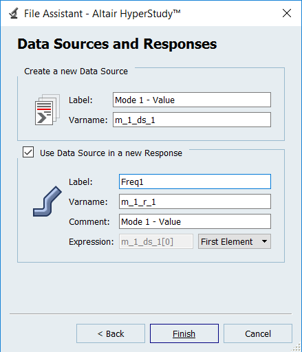
Figure 6.
-
Define the following options and click
Next.
-
Create the Volume output response.
- Click Evaluate to extract the response values.
Run Optimization
-
Apply an objective on the Volume output response.
- Click Add Goal.
- In the Apply On column, select Volume (r_2).
- In the Type column, select Minimize.

Figure 7. -
Apply a constraint to the Freq1 output response.
- Click Add Goal.
- In the Apply On column, select Freq1.
- In the Type column, select Constraint.
- deterministic
- In column 1, select >= (less than or equal to).
- In column 2, enter 32.

Figure 8. -
Click the Iteration History tab to monitor the progress
of the Optimization iteration.
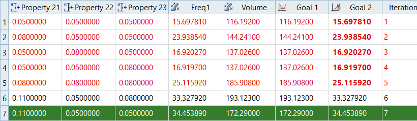
Figure 9.
Run DOE
Run a DOE to find the the true best design.
-
Click the Levels tab, and change the Levels for each
input variable to 5.
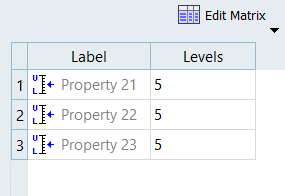
Figure 10. -
Sort run data based on the Volume (which was to be minimized) by right-clicking
on the Volume column and selecting Sort down from the context menu. The lowest
volume design which satisfies the constraint (frequency > 32) is the same as
that found by the optimizer.
Note: The DOE took 125 solver calls to exhaust all combinations, whereas the Optimization found it in 8 solver calls.
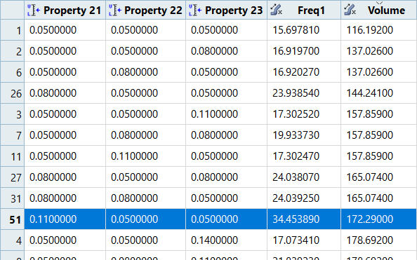
Figure 11.