HS-4420: Optimization Study of a Spherical Impactor
Learn how to perform an advanced study that has both size and shape input variables
on a RADIOSS finite element model.
Before you begin, copy the model files used in
this tutorial from <hst.zip>/HS-4420/ to your working
directory.
The steps taken in this tutorial demonstrate how to analyze the input variables in
order to identify the most important variables and how to do an Optimization. The
objective of the Optimization is to minimize the maximum acceleration of the
impactor, while keeping maximum displacement lower than 16 mm.
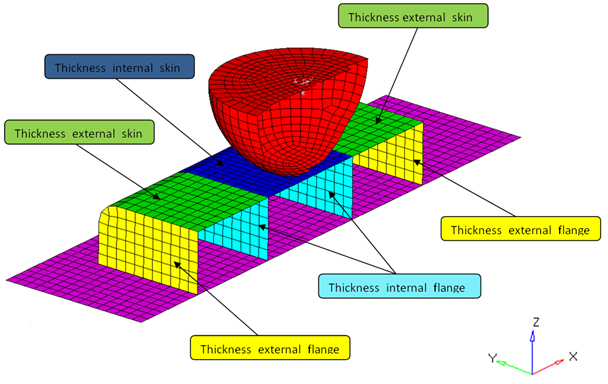
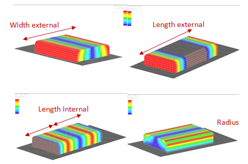
This model simulates the dynamic impact of a sphere with an initial velocity on a
box. There are eight variables: four size variables, which are four box thickness,
and four shapes variables. Figure 1. Size Variables Figure 2. Shape Variables
Export Shape Parameterization from HyperMesh
Start HyperMesh Desktop.
In the User Profiles dialog, change the user profile to
RADIOSS.
Open model.
From the menu bar, click File > Open > Model.
In the Open Model dialog, open the
impactor.hm file.
The impactor.hm database has the RADIOSS analysis
setup, and the shapes have already been created. You must export the shapes
variables so that they are included in the template file.
Create shapes.
From the Tool page, click shape.
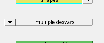
Go to the desvar subpanel and switch single
desvars to multiple desvars.
Figure 3.
Enter the following values:
initial value: 0
lower bound: -1
upper bound: 1
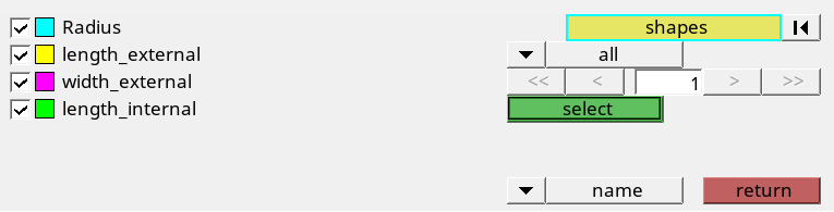
Click the shapes collector.
Figure 4.
Select all of the shapes.
Figure 5.
Click select.
Click create.
A shape design variable is created for each shape.
Optional: Animate or visualize shapes.
Click animate.
In the Deformed panel, click linear or
modal to animate the shape variables in the
modeling window.
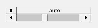
While the shape is animating, you can adjust the animation speed by
moving the slider as indicated in the image below.
Figure 6.
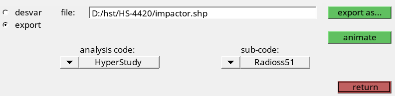
Export and save shapes.
Go to the export subpanel.
For analysis code, select HyperStudy.
For sub-code, select Radioss51.
In the File field, enter impactor.shp.
Click export as.
In the Save As dialog, navigate to your working
directory and save the file as impactor.shp.
impactor.shp: Grid perturbation vector data read by
impactor.radioss51.node.tpl
Exit HyperMesh desktop.
Create Base Input Template
In this step, create the base input template in HyperStudy.
Start HyperStudy.
From the menu bar, click Tools > Editor.
The Editor opens.
In the File field, open the impactor_0000.rad file.
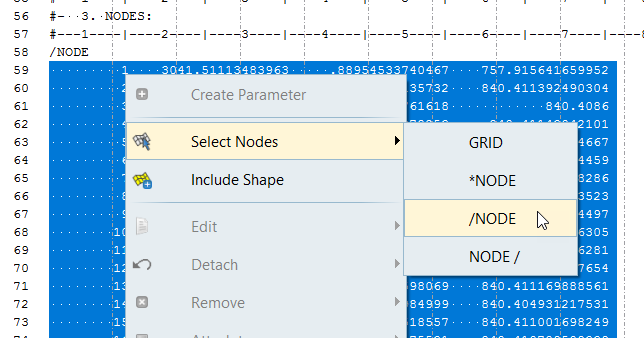
Right-click anywhere in the editor and select Select Nodes > /NODE from the context menu.
All of the /NODE cards in the impactor_0000.rad
file highlight. Figure 8.
Right-click on the highlighted cards and select Include
Shape from the context menu.
In the Shape Template dialog, open the
impactor.radioss51.node.tpl file.
The shape variables are created and the grid is replaced by the
parameter file (which contains the grid parameterized by the shapes) exported
during the step Export Shape Parameterization from HyperMesh.
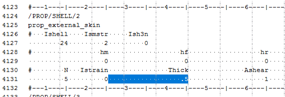
Create parameter.
Select the thickness value for
prop_external_skin.
In a RADIOSS deck, each field within a card is 20 characters
long.
Tip: To assist you in selecting 20-character
fields, press Control to activate the
Selector (set to 20 characters) and then click the
value. Figure 9.
Right-click on the highlighted fields and select Create
Parameter from the context menu.
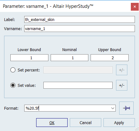
The Parameter: varname_1 dialog
opens.
In the Label field, enter
th_external_skin.
Modify bounds.
Lower Bound: 1.0
Nominal value: 1.0
Upper Bound: 2.0
In the Format field, enter %20.5f.
Click OK.
Figure 10.
Define three more input variables for thickness using the information provided
in Table 1:
Table 1.
Input Variable
Label
Lower Bound
Nominal Value
Upper Bound
Format
prop_internal_skin
th_internal_skin
1.0
1.0
2.0
%20.5f
prop_external_flange
th_external_flange
1.0
1.0
2.0
%20.5f
prop_internal_flange
th_internal_flange
1.0
1.0
2.0
%20.5f
Click OK to close the Editor.
In the Save Template dialog, navigate to your working
directory and save the file as impactor.tpl.
Perform the Study Setup
Start a new study in the following ways:
From the menu bar, click File > New.
On the ribbon, click .
In the Add Study dialog, enter a study name, select a
location for the study, and click OK.
Go to the Define Models step.
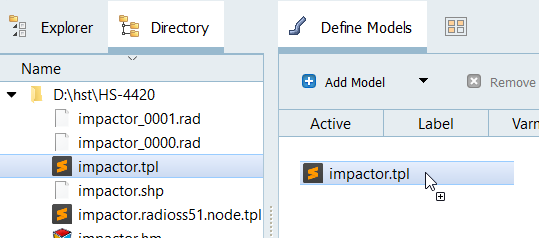
Add a Parameterized File model.
From the Directory, drag-and-drop the impactor.tpl
file into the work area.
Figure 11.
In the Solver input file column, enter
impactor_0000.rad.
This is the name of the solver input file HyperStudy writes during the evaluation.
In the Solver execution script column, select
RADIOSS.
In the Solver input arguments column, enter -nproc
4 after ${file}.
Define a model dependency
Click Model Resources.
The Model Resource dialog opens.
Select Model 1 (m_1).
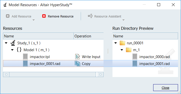
Click Resource Assistant > Add File.
In the Select File dialog, navigate to your
working directory and open the impactor_0001.rad
file.
Set Operation to Copy.
Click Close.
Figure 12.
Click Import Variables.
Eight input variables are imported from the
impactor.tpl resource file.
Go to the Define Input Variables step.
Review the input variable's lower and upper bound ranges.
Perform Nominal Run
Go to the Test Models step.
Click Run Definition.
An approaches/setup_1-def/ directory is created
inside the study Directory. The
approaches/setup_1-def/run__00001/m_1 directory
contains the input file, which is the result of the nominal run.
Create and Evaluate Output Responses
In this study, you want to analyze the maximum acceleration and the maximum
displacement observed by the box. This study is a function of the time; you need to extract
the maximum of each output response vector over time.
Go to the Define Output Responses step.
Create a file source for time.
Click the Data Sources tab.
From the Directory, drag-and-drop the impactorT01
file, located in
approaches/setup_1-def/run__00001/m_1, into the
work area.
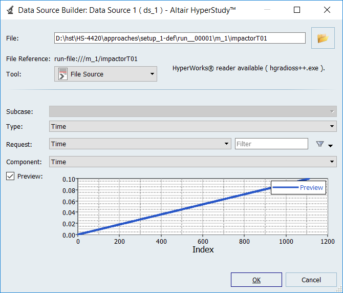
The Data Source Builder dialog
opens.
For Tool, select File Source.
Define the following options:
Type: Time
Request: Time
Component: Time
Click OK.
Figure 13.
Create a second file source for impactor acceleration along the Z axis by
repeating step 2 with the following changes:
Type: Node/TH_node_sphere
Request: 4206 rigid_sphere_4206
Component: AZ-Z Acceleration
Create a third file source for impactor displacement along the Z axis by
repeating step 2 with the following changes:
Type: Node/TH_node_sphere
Request: 4206 rigid_sphere_4206
Component: DZ-Z Displacement
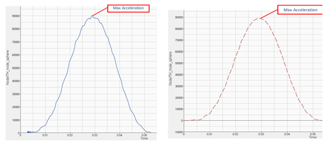
All of the result vectors for the Max_Acceleration output response are
created. The left graph seen in Figure 14 has some noise. To eliminate the noise, you will use a filter
and work on the filtered output response as demonstrated in the right graph shown in
Figure 14. Figure 14.
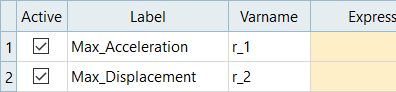
Add two output responses.
Click the Define Output Responses step.
Click Add Output Response twice.
In the work area, change the labels for the output responses to
Max_Acceleration and
Max_Displacement.
Figure 15.
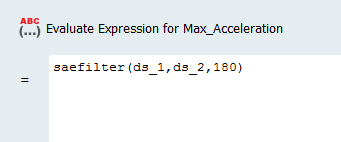
Define the Max_Acceleration output response.
In the Expression column of the output response Max_Acceleration, click
(...).
In the Expression Builder, click the Functions
tab.
From the list of functions, select
saefilter.
This function will apply a filter to the acceleration vector.
Click Insert Varname.
The function saefilter(,,) appears in the Evaluate Expression
field. You can now add the time vector and the acceleration vector as
arguments to the function, with a class parameter of 180.
In the Evaluate Expression field, enter
(ds_1,ds_2,180) in the saefilter
function.
Figure 16.
To calculate the max of the expression, add the max function to the
beginning of the expression.
The expression should read:
max(saefilter(saefilter(ds_1,ds_2,180)0)).
To express the result in G, divide the max of the expression by
9810.
The expression should read:
max(saefilter(ds_1,ds_2,180)/9810).
Click OK.
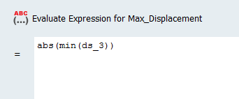
Define the Max_Displacement output response.
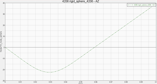
Optional: Plot the displacement with respect to the time, to obtain the curve
illustrated below:
Figure 17.
In the Expression column of the output response Max_Displacement, click
(...).
In the Expression Builder, click the Functions
tab.
From the list of functions, select abs.
Click Insert Varname.
The function abs() appears in the Evaluate Expression
field.
From the list of functions, select min.
Click Insert Varname.
The expression should now read,
abs(min()).
In the Evaluate Expression field, enter ds_3 in
the min function.
Figure 18.
Click OK.
Click Evaluate to extract the response values.
Run Screening DOE Study
Reduce the number of input variables by running a screening experiment.
The model has 8 variables which may lead to high computation times for direct
optimization or even for creating a response surface. A full factorial experiment with 8
factors at 2 levels will require 28 (256) runs and with 3 levels, it will increase to
6561 runs. You will try to screen out some input variables by first doing a Fractional
Factorial screening DOE.
Add a DOE.
In the Explorer, right-click and select
Add from the context menu.
In the Add dialog, select
DOE and click OK.
Go to the DOE 1 > Specifications step.
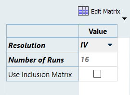
In the work area, set the Mode to Fractional
Factorial.
In the Settings tab, set Resolution to IV.
Note: Resolution IV enables an estimate of main effects unconfounded by
two-factor interactions. It also enables an estimate of two-factor
interaction effects, which may be confounded with other two-factor
interactions. Figure 19.
Verify that the Number of Runs is set to 16.
Click Apply.
Go to the DOE 1 > Evaluate step.
Click Evaluate Tasks.
Go to the DOE 1 > Post-Processing step.
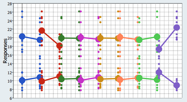
Click the Linear Effects tab to review the linear
effects.
Observe the main effect of the input variables on both output responses. Figure 20.
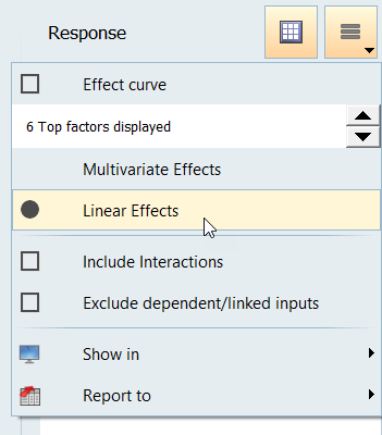
Click the Pareto Plot tab, then use the
Channel selector to select both of the output
responses.
A linear effects plot and a pareto plot with the Linear
Effects option enabled (shown in Figure 21) provide the same
information. However, with a pareto plot, you can use a statistical measure
(that is, the 80-20 rule) to decide which input variables are more significant
and which input variables can be neglected. Figure 21.
For this tutorial, you will use the 80/20 rule to eliminate input
variables that are not significant to the study. The 80/20 rule is a Pareto
principle that proposes 80% of the total effects comes from only 20% of the
variables.
Note: You should also use other practices to eliminate input
variables that you feel should be taken in consideration.
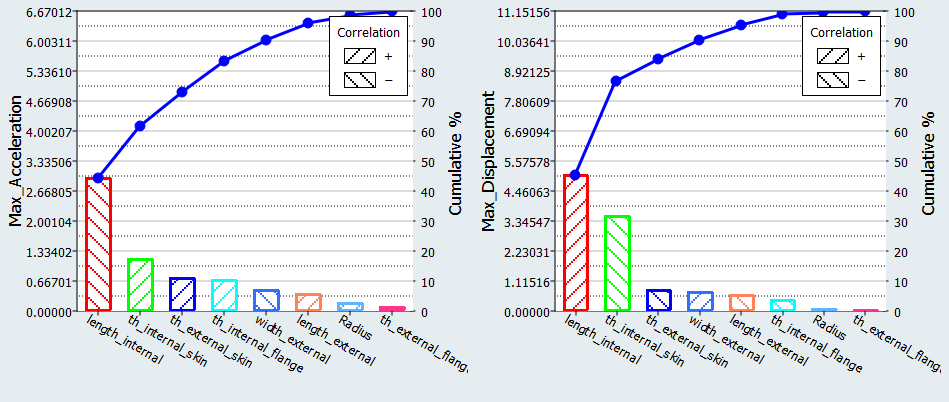
For screening purpose, you can see which input variables contribute to 80% or
more of the given output response. In Figure 22 you can see the
following:
For Max_Acceleration, the input variables length_internal,
th_internal_skin, and th_external_skin contribute to 80% of the linear
effect.
For Max_Displacement, the input variables length_internal and
th_internal_skin fall under the 80/20 rule.
For n responses, you can list out the input variables that follow the 80/20
rule, and take union of the sets. In this case, the input variables that follow
the 80/20 rule include: length_internal, th_internal_skin, and th_external_skin.
This narrows your list to three significant input variables. Figure 22.
Run DOE Study for Approximation
Since this optimization is based on response surfaces, a
central composite experiment will be used, which will create a 2nd order response
surface.
Add a DOE.
In the Explorer, right-click and select
Add from the context menu.
In the Add dialog, select
DOE and click OK.
Go to the DOE 2 > Definition > Define Input Variables step.
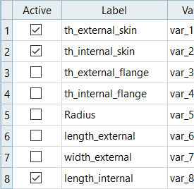
In the Active column, keep only the three significant input variables active
(established in the step:Post-Process the Screening DOE Study), and clear the
corresponding checkboxes for all other input variables.
Figure 23.
Go to the DOE 2 > Specifications step.
In the work area, set the Mode to Central
Composite.
Click Apply.
Go to the DOE 2 > Evaluate step.
Click Evaluate Tasks.
Run DOE Study for the Validation Matrix
Other points will be used to check the quality of the approximation.
The points will be defined by a new DOE. In this DOE study, a Latin HyperCube of 10
runs will be used.
In the Specifications step, set the Mode to Latin
HyperCube.
In the Settings tab, change the Number of Runs to
10.
Create Fit
Add a Fit.
In the Explorer, right-click and select
Add from the context menu.
In the Add dialog, select
Fit and click OK.
Import matrix.
Go to the Fit > Specifications step.
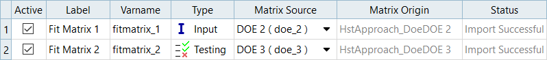
Click Add Matrix twice.
Define Fit Matrix 1 and Fit Matrix 2 by selecting the options indicated
in Figure 24.
Figure 24.
Click Apply.
Review input variables.
Go to the Fit > Definition > Define Input Variables step.
Only the length_internal, th_internal_skin, and th_external_skin input
variables should be active.
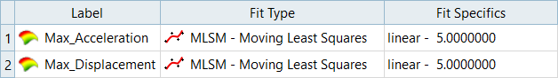
Define specifications.
Go to the Fit > Specifications step.
In the work area, Fit Type column, select Moving Least
Squares (MLSM) for all output responses.
Figure 25.
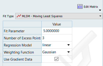
In the Settings tab, verify that Regression Model is set to
Linear for all output responses.
Note: It is advisable to start with lowest order and increment it in
case model Residuals and Diagnostics do not look feasible.
Figure 26.
Click Apply.
Go to the Fit > Evaluate step.
Click Evaluate Tasks.
To assess the accuracy of the regression equations, go to the Fit > Post-Processing step and click the Residuals and
Diagnostics tab.
To review the output response curves and surfaces, click the
Trade-Off tab.
In the Trade-Off 3D tab, use the Channel selector to plot input variables and
output responses. The values for the input variables which are not plotted are
modified in the top frame (Inputs). Move the sliders in the Value column to
modify the other input variables, while studying the output response throughout
the design space.
Run Optimization
Add an Optimization.
In the Explorer, right-click and select
Add from the context menu.
In the Add dialog, select
Optimization and click OK.
Modify input variables.
Go to the Optimization > Definition > Define Input Variables step.
In the Active column, clear the checkboxes for all input variables
except length_internal, th_internal_skin and th_external_skin.
Go to the Optimization > Definition > Define Output Responses step.
Click the Objectives/Constraints - Goals tab.
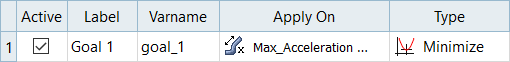
Apply an objective on the Max Acceleration output response.
Click Add Goal.
In the Apply On column, select Max
Acceleration.
In the Type column, select Minimize.
Figure 27.
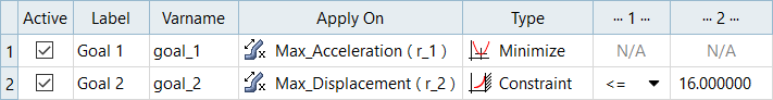
Apply a constraint on the Max_Displacement output response.
Click Add Goal.
In the Apply On column, select
Max_Displacement.
In the Type column, select Constraint.
In column 1, select <= (less than or equal
to).
In column 2, enter 16.
Figure 28.
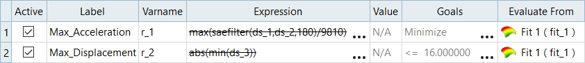
Modify evaluation source.
Click the Define Output Responses tab.
In the Evaluate From column, select Fit 1
(fit_1) for both output responses.
Figure 29.
Go to the Optimization > Specifications step.
In the work area, set the Mode to Genetic Algorithm
(GA).
Click Apply.
Go to the Optimization > Evaluate step.
Click Evaluate Tasks.
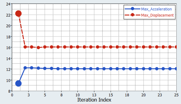
The program will optimize the design that minimizes the maximum
acceleration while keeping the displacement of node 35527 smaller than
16.
Click the Iteration Plot tab to monitor the Optimization
iteration.
Figure 30.
Click the Iteration History tab to review a table of
each iteration.
The iterations that do not respect the constraint are displayed red, the
optimal design is displayed green.
Run Verification
In this step, you will run a Verification to check if the solution found by the
approximation is close to the solver results.
Add a Verification.
Go to the Optimization > Evaluate step.
Click Verify.
Figure 31.
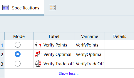
Go to the Verification > Specifications step.
In the work area, set the Mode to Verify Optimal.
Figure 32.
Click Apply.
Go to the Verification > Evaluate step.
Click Evaluate Tasks.
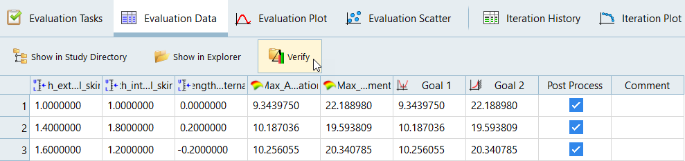
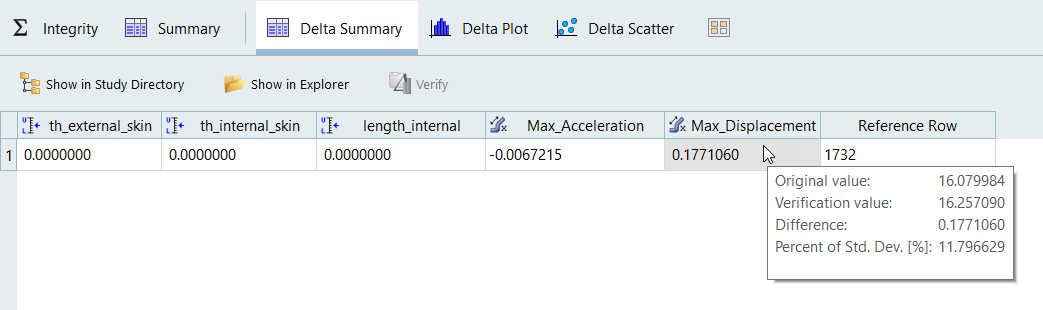
Go to the Verification > Post-Processing step.
Click the Delta Summary tab.
Hover your cursor over the value of the Max-Displacement
column to review the difference between the fit predicted values (original
value) and the solver run results (verification value).
As shown in Figure 33,
there is a small difference in displacements. Figure 33.

 .
.