HS-4425: Multi-Objective Shape Optimization Study

Perform a multi-objective Optimization study, and search for the Pareto front that minimizes both volume and maximum displacement.

Before you begin, complete HS-4000: Optimization Method Comparison: Arm Model Shape Optimization or import the HS-4000.hstx archive file, available in <hst.zip>/HS-4425/.
In this tutorial you will be using MOGA with a Fit to save time.
Note: If a Fit was not available, GRSM would be the suggested method to use in order to solve a MOO problem. MOO problems require many evaluations, therefore GRSM is more efficient than MOGA.

Run Multi-Objective Shape Optimization

  1. Add an Optimization.
    1. In the Explorer, right-click and select Add from the context menu.
    2. In the Add dialog, select Optimization and click OK.
  2. Modify input variables.
    1. Go to the Optimization 7 > Definition > Define Input Variables step.
    2. In the work area, Active column, clear the radius_1, radius_2 and radius_3 checkboxes.
  3. Go to the Optimization 7 > Definition > Define Output Responses step.
  4. Click the Objectives/Constraints - Goals tab.
  5. Apply an objective on the Volume and Max_Disp output responses.
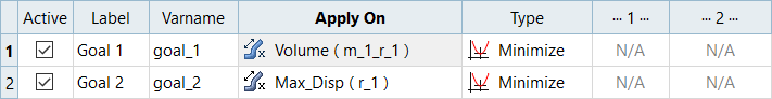
    1. Click Add Goal twice.
    2. In the Apply On column, select the following:
      • Goal 1: Volume
      • Goal 2: Max_Disp
    3. In the Type column, select Minimize.


    Figure 1.
  6. Click the Define Output Responses step, and change the Evaluate From column to Fit - RBF (fit_4) for Volume, Max_Stress, and Max_Disp.
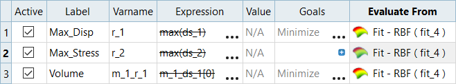

    Figure 2.
  7. Go to the Optimization 7 > Specifications step.
  8. In the work area, set the Mode to Multi_Objective Genetic Algorithm (MOGA).
  9. Click Apply.
  10. Go to the Optimization 7 > Evaluate step.
  11. Click Evaluate Tasks.
    HyperStudy stops MOGA after 50 iterations, and performs a total of 13317 analyses. The Pareto front of the last iteration contains 408 points.
  12. Go to the Optimization > Post-Processing step.
  13. Click the Optima tab.

    The Pareto front of Objective 2 versus Objective 1 is displayed in the plot.

    The goal of this study was to minimize both Volume (Objective 1) and Max_Disp (Objective 2). The Pareto plot shows all of the non-dominated solutions. A non-dominated solution is a solution which can no longer improve one objective without deteriorating another. You can see that minimizing Objective 1 will increase Objective 2, and minimizing Objective 2 will increase Objective 1. According to these results, you must decide what would be the optimal solution. For instance, the Pareto plot may allow a compromise solution to be selected somewhere in the middle.
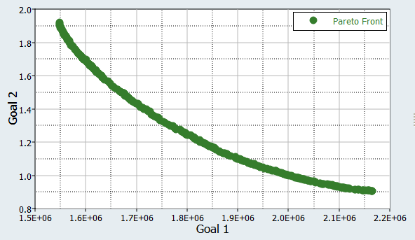


    Figure 3.