HS-4550: Multi-physics Optimization of Aircraft Radome Using HyperStudy Fit Models
In this tutorial, you will perform a multi-physics optimization using HyperStudy Fit models instead of solver models.
Before you begin, copy the model files used in this tutorial
from <hst.zip>/HS-4550/ to your working directory.
The fit approximations for each physical analysis (Electromagnetic, Structural, Bird strike) have been built in prior studies and exported in portable pyfit format, which can be grouped within a single study.
Perform Study Setup Definition
-
Start a new study in the following ways:
- From the menu bar, click .
- On the ribbon, click
 .
.
-
Add a HyperStudy Fit model.
- From the Define Models step, click Add Model.
- In the HyperStudy - Add dialog, select HyperStudy Fit model and click OK.
- In the Label column, change the name to Structural.
-
In the Resource column, click
 .
.
- In the HyperStudy - Load model resource dialog, select fit_Structural_analysis_OS.pyfit and click Open.

Figure 1.The HyperStudy Fit model is created and a Python Fit Solver is automatically populated in the Solver Execution Script column. -
Add two more HyperStudy Fit models by repeating step 3, except change the label and resource for each model as
shown in Table 1.
Table 1. Label Resource Bird strike fit_Birdstrike_analysis_Radioss.pyfit Electromagnetics fit_ElectroMagnetic_analysis_FEKO.pyfit 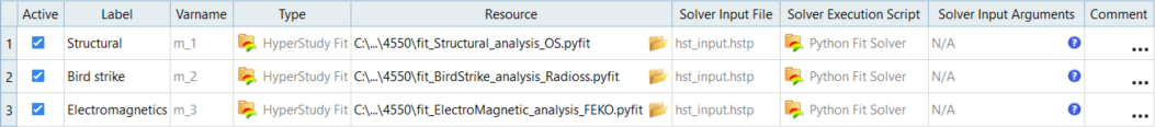
Figure 2. -
For the Thickness_Foam variable, verify the mode is set to
Continious.
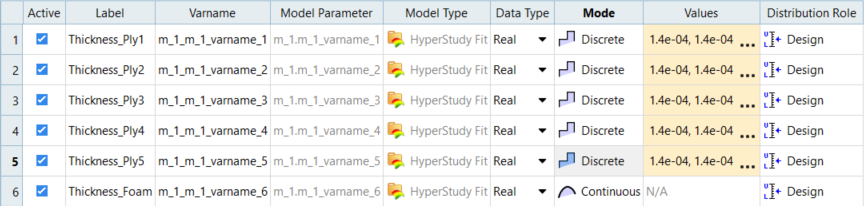
Figure 3. -
Edit values for all Thickness_Ply variables.
-
For Thickness_Ply1, click
 in the Values column.
- For Step Size, enter 1.40e-04 and click Set.
- Click OK.
- Repeat step 9 for the remaining Thickness_Ply variables.
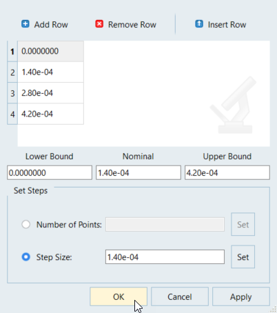
Figure 4. -
For Thickness_Ply1, click
-
Link variables to ensure consistent variations in different analysis.
-
For ply1, click in the Expression column.
-
In the Expression Builder dialog, enter
m_1_m_1_varname_1*1000 in the Evaluate
Expression field.
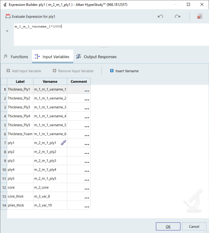
Figure 5.
The variables of the Bird strike and Electromagnetics models are linked to the variables of the Structural model and they will change accordingly within the evaluations.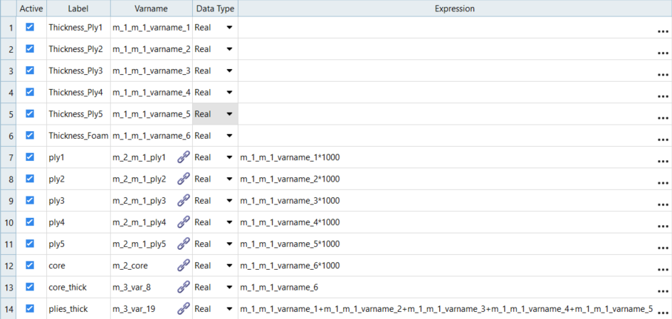
Figure 6. -
For ply1, click
-
Define the constraint.
-
In the Left Expression column, click .
- In the Expression Builder dialog, enter m_1_m_1_varname_1+m_1_m_1_varname_2+m_1_m_1_varname_3+m_1_m_1_varname_4+m_1_m_1_varname_5 in the Evaluate Expression field.
- Click OK
- Set Comparison to >=.
- For Right Expression, enter 1.4e-04.

Figure 7. -
In the Left Expression column, click
-
For Constraints, select 4 and click
Add.
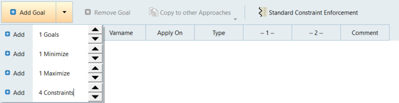
Figure 8.