# Create a model
m = sliding_block("lugre1")

# Define a custom simulation function
def mySlidingBlockSimulation (m):
m.simulate (type="DYNAMICS", end=4, dtout=.01)
m.lugre.mus=0.5
m.simulate (type="DYNAMICS", end=8, dtout=.01)

# Perform a custom simulation on the model
mySlidingBlockSimulation (m)
# Initialize a few variables: duration for each simulation, # simulations done, a string
dur = 4.0
num_simulations = 0
textstr = '$\mu=$'# Read the model
m = sliding_block()
################################################################################ Loop until user asks you to stop ################################################################################while True:
# Get a value for mu static or a command to stop
mus = raw_input ("Please enter a value for mu static or stop: ")
if mus.lower ().startswith ("s"):
breakelse:
num_simulations +=1
# Apply the value of mu static the user provided and do a simulation
m.lugre.mus=mus
run = m.simulate (type="DYNAMICS", returnResults=True, duration=dur, dtout=0.01)
textstr += ', %.2f '%(m.lugre.mus)
# Get the request time history from the run object
disp = run.getObject (m.r1)
velo = run.getObject (m.r3)
force = run.getObject (m.r2)
################################################################################ Plot some interesting results ################################################################################import matplotlib.pyplot as plt
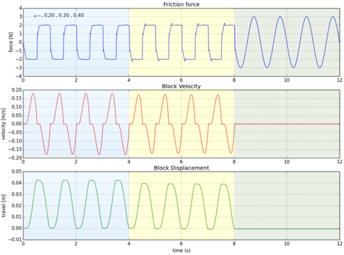
# Friction force vs. Time
plt.subplot (3, 1, 1)
plt.plot (force.times, force.getComponent (3))
plt.title ('Friction force')
plt.ylabel ('force [N]')
plt.text (0.4, 3, textstr)
plt.grid (True)
# Block Velocity vs. Time
plt.subplot (3, 1, 2)
plt.plot (velo.times, velo.getComponent (3), 'r')
plt.title ('Block Velocity')
plt.ylabel ('velocity [m/s]')
plt.grid (True)
# Block Displacement vs. Time
plt.subplot (3, 1, 3)
plt.plot (disp.times, disp.getComponent (3), 'g')
plt.title ('Block Displacement')
plt.xlabel ('time (s)')
plt.ylabel ('travel [m]')
plt.grid (True)
plt.show()
The results of this simulation are shown below.