Best Practices for Running 3D Contact Models in MotionSolve

MotionSolve can detect and handle contact between graphic entities that represent solids.

The graphics may be defined in three ways:

Analytically for simple shapes such as spheres and frusta
As CAD geometry in their native format
As triangular meshes

Regardless of how they are created, all geometry (except for sphere-to-sphere and sphere-to-mesh contact) is eventually converted to a mesh and contact between meshes is computed during the simulation.

This section summarizes contact strategies that will help you experience successful simulation.

Model Best Practices

Constraints vs. Contacts
Use Joints, Joint Primitives and other constraints instead of Contact when possible. The former are much more efficient and will save simulation time. Use contacts only where they are needed.
Use analytical descriptions or CAD geometry to define solids where possible
Analytical descriptions are guaranteed to be solid, however they can be used only when the geometry is simple. Use these where you can.

If the use of analytical geometries is not possible, use native CAD geometry. CAD geometries are usually available and they can be simply reused. MotionView can import all the common CAD geometry formats. It is easy to check that the CAD descriptions define a solid. MotionView performs numerous checks when importing CAD geometry. If errors are found they are reported in the message window.

If neither analytical nor CAD descriptions are not available, then you should consider using other sources of input such as meshes defined by an FE pre-processor, STL files or Wavefront OBJ files. MotionView will check this data too to make sure it defines solid bodies.
Visualize the mesh in MotionView to identify inappropriate meshes

The mesh representing a rigid body must have an appropriate element size.

The mesh should accurately capture the curvature of the geometry that is going to be in contact. Care should be taken to minimize the effects of tessellation on contact response. Meshes with small elements usually produce more accurate results but at the expense of more computation time. Figure 1 below illustrates "good" and "bad" meshes.

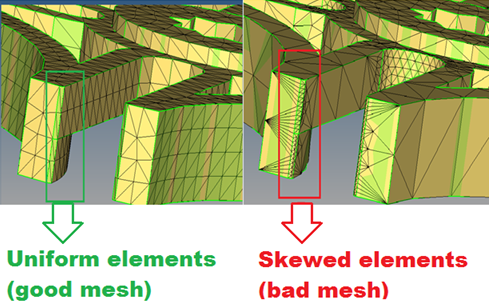
Figure 1. An Example of Normals Defined "Inward" (blue) vs "Outward" (red)

Mesh triangles must maintain uniformity in elements size.

This generates accurate contact forces. Don't use a mix of coarse and fine mesh in a same graphics. See Figure 2.

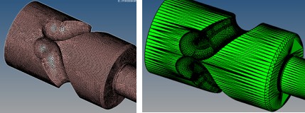
Figure 2. An Example of Uniform (good) and Non-uniform (bad) Elements in a Mesh

Meshes must have outward facing normals.

The "outward" side is defined as the side where contact will occur. Similarly, "inward" side is defined as the side where the material exists in the closed volume. Triangles with outward normals are colored red and triangles with inward normals in blue. See Figure 3.

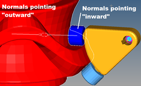
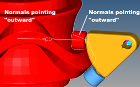Figure 3. An Example of Normals Defined "Inward" (blue) vs "Outward" (red)

Such a situation will be encountered ONLY when older models containing the geometry in H3D files are provided as input. Models created with 14.0 will have ALL triangles for a geometry pointing inwards (blue) or outwards (red).

You can simply flip the normals with one keystroke. Use the option "Material Inside" option in MotionView to flip the direction of the surface normals to the direction of expected contact.
Understand the diagnostics MotionView provides when faulty geometry is provided
MotionView performs extensive checks on the geometries that are defined for Contacts and it will identify the following defects in geometry:

The mesh is not closed and it does not enclose a volume.

The open areas are highlighted. See Figure 4 for an example.

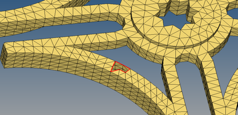
Figure 4. An Example of an Open Volume Mesh That Should be Avoided

The mesh contains T-connections or T-junctions

A T-junction is a spot where two polygons meet along the edge of another polygon. T-junctions do not occur in solids. See Figure 5 for examples.

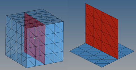
Figure 5. An Example of a T-connection in a Mesh
Use MotionView to generate good quality tessellations for contact
You can use the Control mesh coarseness for contacts option in MotionView to generate good quality tessellations. This option is designed to provide a uniform mesh needed for contact simulation. See Figure 6 to find out where the options are available in the user interface.

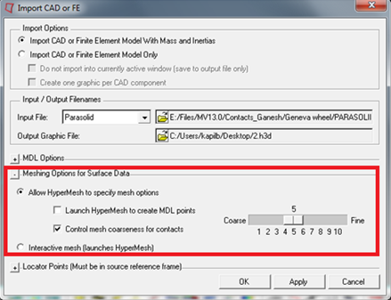
Figure 6. MotionView Allows You to Control the Mesh Coarseness while Importing Geometries

Start with the default setting of "5" coarseness slider bar. In most cases, this setting would give a suitable uniform mesh appropriately capturing the curvatures.

Review the imported graphics; especially those bodies that would be used in contacts. If not satisfied with the size of the mesh, re-import the CAD using a finer option (higher number) in the coarseness slider bar. Below are a few points to remember while refining the mesh
- The number of triangles that are in contact affects contact performance. The portion of the mesh not in contact neither affects the speed nor the accuracy of the contact. So, it is OK to have a fine mesh for the entire component, even though only a very small part of it is in contact. There will be an initial setup cost, but the simulation speed is not overly affected.
- Care has to be taken with very large CAD files as it might take a large amount of time. If possible, make sure the input CAD only has the bodies that are going to be involved in contacts.
- Try and predict the features of the body that are most probably going to engage in the contact. Ensure these particular features are well captured in the output mesh.
- Make sure that the curvature of the surface that is intended for contacts is accurately captured by an appropriately small element size. Also make sure that the mesh in that particular region has all the qualities of a good fundamental mesh listed earlier.
- If the resulting mesh has open edges, a warning will be generated in the message log. This indicates the mesh does not enclose a volume
  If the above method of refinement does not yield mesh as expected, use the Interactive Mesh option in HyperMesh to mesh the geometries.
Solving legacy models with CAD graphics
Legacy models may have geometries that are not appropriate for the methods used in MotionSolve 14.0. A good general solution is to regenerate the H3D graphics for contact once again by using the new tools and features in the Import CAD tool in MotionView.

If this is not possible, go ahead and use the legacy geometry. MotionView now supports a geometry cleaning process. This process systematically checks the geometry for various possible errors and fixes them. The geometry cleanup process is explained in Appendix-I.
Handling complex geometries
In rare occasions, you may see that the contact setup in MotionSolve is expensive. In such uncommon scenarios, split the contact geometry to separate graphics and use these for contact. See Figure 7 for an illustration.

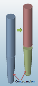
Figure 7. Splitting a Large Geometry into Separate Parts

Contact Properties

MotionView provides a fairly good set of default values for contact properties. The default values for contact properties in MotionView are summarized in the table below.

Impact Model

Normal Force	Friction Force
Stiffness = 1000 N/mm	μ_static = 0.2
Damping = 0.1 N s / mm	μ_dynamic = 0.2
Exponent = 2.1	Stiction Transition Velocity = 0.1 N s / mm
Penetration Depth = 0.1 mm	Friction Transition Velocity = 0.2 N s / mm

Poisson Model

Penalty = 5000 N/mm

Restitution Coefficient = 0.8

Normal Transition Velocity = 1 mm/s

Volume Model

I/J body Bulk Modulus = 1.6E5 N/(mm)²

I/J Body Shear Modulus = 1.6E5 N/(mm)²

I/J Body Layer Depth = 1000 mm

Exponent = 2.1

Damping = 1 N/mm

We recommend that you change these only if the units you are using for your model is different or if the default set is somehow ineffective. General guidelines for changing these parameters are below.

Contact Stiffness
Initially set "low" values for stiffness (penalty) for the normal force. This will enable fast simulations. Review the contact overview table for the maximum penetration seen in the simulation result. If these are higher than expected, increase the stiffness. While using large values for stiffness (penalty) if the contact force is noisy, reduce the simulation step size.
Contact Damping / Coefficient of Restitution
Set damping to be about 0.1%-1% of the stiffness or set the coefficient of restitution around 0.4. Models with no damping are prone to undamped high frequency vibration, which will lead to small step sizes. Conversely, models with high damping can also be problematic as the damping force can dominate the overall response.
Contact Friction
Start your modeling with Contact friction set to Disabled. Once the simulation is successful with just normal forces (reasonable penetration and normal force values) then contact friction should be turned ON.

Do not use small values for the parameters Stiction Transition Velocity and Friction Transition Velocity. Small values will slow down the simulation speed. Approximately 1mm/sec is a good value.

If the addition of frictional force causes numerical difficulties or simulation slowdowns, gradually increase the values for the transition velocities and/or reduce the coefficients of friction. Avoid large values for μstatic and μdynamic.
Contact and Statics / Quasi-statics
In general, it is a good idea to have a slight initial penetration between contacting surfaces when performing statics. This will ensure that the Newton-Raphson iteration algorithm does not compute large changes in the direction of the contact.

Avoid neutral equilibrium situations. If you know that your model has neutral equilibrium situations, increase STABILITY.
Handling Intermittent Contacts
When there are many intermittent contacts in your model, it is a good idea to use the Find precise contact event option in the Advanced tab. This will ensure that contacts are not missed or that penetration is not too high. See Figure 8.

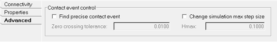
Figure 8. Advanced Tab in MotionView for Modeling 3D Contacts
- A maximum step size of 1e-4 is a good initial setting for contact simulations
- Use appropriate units in model based on dimension of geometry length. While modeling the ball bearing of a hand drill mm units will be appropriate than using meter units.

Units Conversion

While using units other than mm for length, and Newton for force, the default stiffness (K) in MotionView for the Impact Model needs to be scaled based on the exponent used.

Contact force F = K*z^e, where z is penetration and e is exponent

Assume K=1000 N/mm and e=2.1

Then the force F = 1000 * z^2.1 N

If the model is defined in SI units, the new stiffness that will generate the same force is calculated as:

F = 1000 * z^2.1 = K * (z÷ 1000)^2.1

∴ K = 1000 * (1000)^2.1 = 1.9953E9

If your model is in SI units, the table below provides parameters equivalent to the MotionView defaults.

Impact Model

Normal Force	Friction Force
Stiffness = 1.9953E9 N/M	μ_static = 0.2
Damping = 100 N s / M	μ_dynamic = 0.2
Exponent = 2.1	Stiction Transition Velocity = 1E-4 M
Penetration Depth = 1E-4 M	Friction Transition Velocity = 2E-4 M

Poisson Model

Penalty = 5E6 N/M

Restitution Coefficient = 0.8

Normal Transition Velocity = 1E-3 M/s

Volume Model

I/J body Bulk Modulus = 1.60E11 Pa

I/J Body Shear Modulus = 1.60E11 Pa

I/J Body Layer Depth = 1 M

Exponent = 2.1

Damping = 1E4 N/M

Master/Main and Secondary Surface
MotionSolve uses the concept of master/main and secondary surfaces while analyzing contacts. The contact forces are calculated only on the master/main surface. The forces on the secondary surface are computed from Newton's third law.

The graphics with a smaller average element size are automatically considered as the master/main surface for contact since this leads to smoother forces. If you want to flip the master/main surface, refine the other graphics used in contact.
Energy Conservation
Contact forces are modeled using a penalty formulation. Unless you take very fine step sizes, the impulse of the forces can be inaccurate. Therefore for impulsive contact, it is not unusual to see energy dissipation or energy gain, even though you may have no damping in your contact. To reduce dissipation, decrease the maximum integration step size so that the contact duration is adequately sampled.

Contact Solutions Evaluation

You must always review the contact response in order to make sure that the system is behaving in the way you intend it to.

Review the contact summary log for the penetrations you are seeing in the simulation. Change the stiffness so that the maximum penetration depth is reasonable
Look at the animation of un-converged results to get a better idea of why the contact may be failing or not behaving as you expect
Review Contact Summary in the MS log file. This option gives a "single view" summary of areas of contact and extent of penetration for the entire simulation
Review the "Contact overview" for unusually high penetrations in unexpected regions.

Commonly Asked Questions

My force output is not smooth. How do I get smoother forces?

Non-smooth contact forces often occur because the contact is not sampled adequately. The usual solution is to reduce the step size so that the contact is adequately sampled. This will provide smoother contact forces. The general guidelines for reducing the step size are explained below.

The contact is modeled as a penalty force. So each contact can be analogous to a mass-spring-damper system. Ignoring damping,

Equivalent mass = M

Equivalent stiffness = K

Frequency of oscillation is:

f = \frac{1}{2 π} \sqrt{\frac{K}{M}}

Recommended integration step: $h = \frac{1}{10 f}$

Consider the following example:

M = 1Kg
K = 50,000 N/m
f = 35.588 Hz
h = 2.8099E-3 s

The plot below shows MotionSolve results for h=2.8099E-3 s and h=5.6199E-3. Note how the results are noisy for the larger h, but are smooth for smaller h.

Figure 10. Mass Displacement

My contact simulations take a long time. How can I improve simulation speed?

There could be multiple reasons why a contact simulation is slow. In this section, we present different strategies for speeding up contact. You can use them in combination as you see fit.

Use force elements instead of contact: If you know where the contacts are going to occur, user force elements to model the contact. These will side step the time consuming contact detection process.
Use constraints instead of contact: Use joints and joint primitives instead of contact when possible. The former are much more efficient and will save simulation time. Use contacts only where they are needed.
Reduce the number of active points in contact: Mesh coarsening may reduce the number of triangles that are actually in contact. This will in turn decrease the time spent in computing the contact kinematics.
Decrease contact stiffness and damping: Initially set "low" values for stiffness (penalty) for the normal force. This will enable fast simulations. Review the contact overview table for the maximum penetration seen in the simulation result. If these are higher than expected, increase the stiffness. While using large values for stiffness (penalty) if the contact force is noisy, reduce the simulation step size. Set damping to be about 0.1%-1% of the stiffness or set the coefficient of restitution around 0.4. Avoid transferring forces between two bodies.
Using multiple cores: Contact detection in MotionSolve is parallelized and MotionSolve uses the maximum number of threads available to your CPU by default. The plot below shows how contact detection scales with the number of processors. Gains of up to 6x may be achieved with this option.

Figure 11. Speed scale-up with increasing number of processors

Which contacts are expensive and consume the most simulation time?

MotionSolve outputs a COF file as output. This file contains a summary of the contact simulation. For each contact, among other information, the time spent in evaluating this contact is printed out. This information is shown here for contact simulation.

Note: Intermediate columns have been removed to make the data fit in the page.

The last column of data contains the CPU time spent in evaluating each contact. Notice the time spent in Contact 8. More time is spent evaluating this contact than all other contacts combined! You should re-examine the contact geometry and contact parameters for Contact 8 to see if you discover anything abnormal or special.

301016,"Contact 16","M-Contact 16",90123, ,90163, ,"MILLIMETER","NEWTON",7.029375
301015,"Contact 15","M-Contact 15",90103, ,90163, ,"MILLIMETER","NEWTON",6.468759
301014,"Contact 14","M-Contact 14",90083, ,90163, ,"MILLIMETER","NEWTON",6.396231
301013,"Contact 13","M-Contact 13",90063, ,90163, ,"MILLIMETER","NEWTON",6.469902
301012,"Contact 12","M-Contact 12",90043, ,90163, ,"MILLIMETER","NEWTON",6.434288
301011,"Contact 11","M-Contact 11",90023, ,90163, ,"MILLIMETER","NEWTON",6.430164
301010,"Contact 10","M-Contact 10",90003, ,90163, ,"MILLIMETER","NEWTON",6.398585
301009,"Contact 9","M-Contact 9",90143, ,90163, ,"MILLIMETER","NEWTON",6.406428
301008,"Contact 8","M-Contact 
8",90123, ,90001, ,"MILLIMETER","NEWTON",172.756276
301007,"Contact 7","M-Contact 7",90103, ,90001, ,"MILLIMETER","NEWTON",7.782117
301006,"Contact 6","M-Contact 6",90083, ,90001, ,"MILLIMETER","NEWTON",7.802998
301005,"Contact 5","M-Contact 5",90063, ,90001, ,"MILLIMETER","NEWTON",7.766806
301004,"Contact 4","M-Contact 4",90043, ,90001, ,"MILLIMETER","NEWTON",7.695826
301003,"Contact 3","M-Contact 3",90023, ,90001, ,"MILLIMETER","NEWTON",7.758897
301002,"Contact 2","M-Contact 2",90003, ,90001, ,"MILLIMETER","NEWTON",7.672547
301001,"Contact 1","M-Contact 1",90143, ,90001, ,"MILLIMETER","NEWTON",7.673137