Custom Simulations
A Simple Example
Just as you can create higher level modeling elements and simplify the task of model building, you can choreograph complex simulations by building your own functions or objects to do so. The previous example shows two sequential simulations being performed.
# Create a model
m = sliding_block("lugre1")

# Define a custom simulation function
def mySlidingBlockSimulation (m):
m.simulate (type="DYNAMICS", end=4, dtout=.01)
m.lugre.mus=0.5
m.simulate (type="DYNAMICS", end=8, dtout=.01)

# Perform a custom simulation on the model
mySlidingBlockSimulation (m)
The model object facilitates more complex custom simulation scenarios. This is explained below.
Complex Simulations with the Model Object
def sliding_block (out_name):
 Line 6: m = Model (output=out_name)
In the line 6 of the example in Build Models with Your Own Modeling Elements, the function sliding_block(), creates a model object, m. The model object is a container that stores the entire model. The model object has several methods that can operate on its contents.
- sendToSolver - Send the model to the Solver
- simulate - Perform a simulation on the model
- save - Store the model and simulation conditions to disk
- reload - Reload a saved model
- control - Execute a CONSUB
- reset - Reset a simulation so the next simulation starts at T=0
You can handle fairly complex simulations using the model methods on the model object.
Here is an extension to the simulation script shown earlier.
- It asks you to specify a μstatic (coefficient of static friction) for the LuGre friction element.
- It applies this value and performs a simulation.
- The process repeats and you can continue providing new values of μstatic.
- The process stops when you issue a STOP command.
- The script then plots some key results for the various values of μstatic you provided and ends the execution.
# Initialize a few variables: duration for each simulation, # simulations done, a string
dur = 4.0
num_simulations = 0
textstr = '$\mu=$'

# Read the model
m = sliding_block()

###############################################################################
# Loop until user asks you to stop #
###############################################################################
while True:

 # Get a value for mu static or a command to stop
mus = raw_input ("Please enter a value for mu static or stop: ")
if mus.lower ().startswith ("s"):
break
else:
num_simulations +=1

 # Apply the value of mu static the user provided and do a simulation
m.lugre.mus=mus
run = m.simulate (type="DYNAMICS", returnResults=True, duration=dur, dtout=0.01)
textstr += ', %.2f '%(m.lugre.mus)

# Get the request time history from the run object
disp = run.getObject (m.r1)
velo = run.getObject (m.r3)
force = run.getObject (m.r2)

###############################################################################
# Plot some interesting results #
###############################################################################
import matplotlib.pyplot as plt

# Friction force vs. Time
plt.subplot (3, 1, 1)
plt.plot (force.times, force.getComponent (3))
plt.title ('Friction force')
plt.ylabel ('force [N]')
plt.text (0.4, 3, textstr)
plt.grid (True)

# Block Velocity vs. Time
plt.subplot (3, 1, 2)
plt.plot (velo.times, velo.getComponent (3), 'r')
plt.title ('Block Velocity')
plt.ylabel ('velocity [m/s]')
plt.grid (True)

# Block Displacement vs. Time
plt.subplot (3, 1, 3)
plt.plot (disp.times, disp.getComponent (3), 'g')
plt.title ('Block Displacement')
plt.xlabel ('time (s)')
plt.ylabel ('travel [m]')
plt.grid (True)

plt.show()

The results of this simulation are shown below.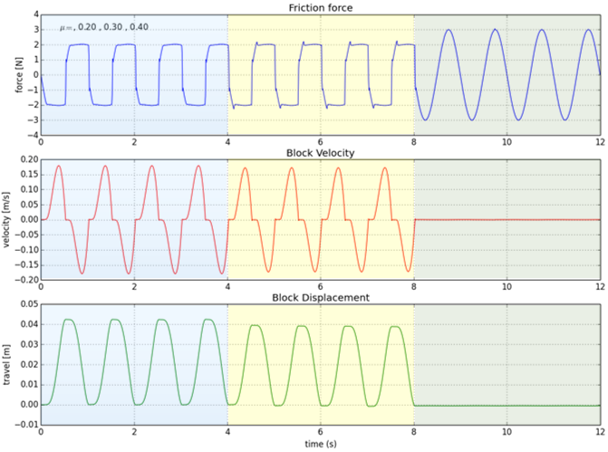
Figure 1.