MV-3010: Optimization using MotionView - HyperStudy
- Perform an optimization study in the MotionView-HyperStudy environment
- Compare the baseline and optimized models
Theory
- The design constraints
- The objective function
- The design variables
Design variables change during optimization. The design variables always have a certain range within which they can be modified. Typical examples of design variables are thickness of shell elements, shape vectors, and masses.
The changes in the design variables cause some change in model responses. Such responses can become either objective function or design constraints. Examples of such responses include displacements and forces.
The response to be minimized or maximized becomes the objective function, while the rest of the responses that need to be within a certain tolerance range become constraints. Only one response can be defined as objective function.
HyperStudy can be used to set-up and perform an optimization study on a MotionView model. You can also use HyperStudy to perform optimization studies involving both linear and non-linear CAE analysis as well as perform optimization of mathematical equations using Templex. HyperStudy creates the input parameter files using Templex and provides iterative changes to them during the optimization process. HyperStudy uses HyperOpt (a general purpose, wrap around software) as the optimization engine to perform optimization, in conjunction with both linear and non-linear CAE analysis software. HyperOpt uses a robust sequential response surface methodology for optimization.
The files needed for this tutorial are hs.mdl, target_toe.csv (used in tutorial MV-3000); Setup.hstudy saved in tutorial MV-3000 and the setup_1-def folder created in tutorial MV-3000.
In the following steps you will perform an optimization study on a front SLA suspension model and determine the optimum coordinate positions of the inner and outer tie-rod points while trying to achieve a target toe curve. The baseline model will then be compared with the optimized model.
Step 1: Optimization Study
-
Click on open file icon,
 , browse to your study directory
and select Setup.hstudy file created in the MV-3000
tutorial.
, browse to your study directory
and select Setup.hstudy file created in the MV-3000
tutorial.
-
Add a new optimization study by doing one of the following:
-
From the Edit menu bar, click the Add Approach
icon,
 , to launch the HyperStudy - Add dialog box.
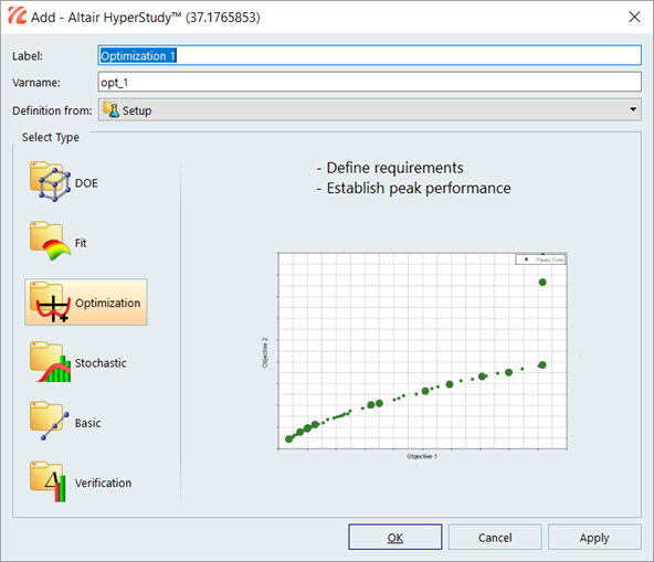
Figure 1. -
Click Next to provide its definition.
Observe that Model and Variables are selected by default.
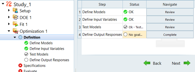
Figure 2.
-
From the Edit menu bar, click the Add Approach
icon,
-
Click Review near Test Models and click Run
Definition to do a test run.
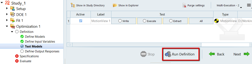
Figure 3. -
Click Next to go to the Select responses.
-
Click
 to Add a goal.
Notice that a goal has been added by default.
to Add a goal.
Notice that a goal has been added by default.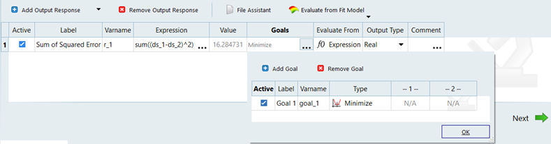
Figure 4. -
Check to make sure that the Evaluate From option is set to
Expression.

Figure 5.
-
Click
-
There aren't any constraints and unused responses in the design, so click
Evaluate and then click Next
to go to Specifications.
Accept the default Optimization Engine: Adaptive Response Surface Method and click Apply and Next. The Maximum iterations and Convergence criteria are specified in the same dialog.
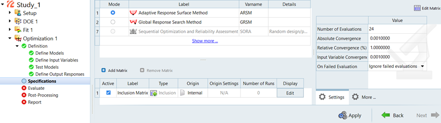
Figure 6. -
Click Evaluate Tasks to start the optimization.
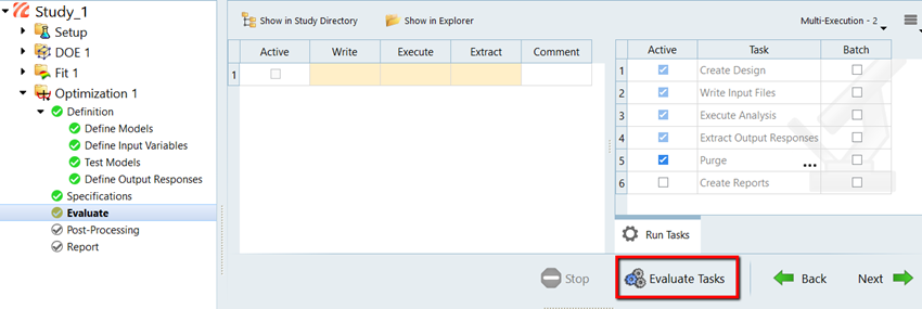
Figure 7.MotionSolve is launched sequentially and the HyperOpt engine attempts to find a solution to the problem.Once the optimization is complete, an Iteration table is created with status of each run. The present study took nine iterations to achieve the target. Browse through the other tabs of this page to get more understanding of the iteration history.
-
From the list on the right side of the GUI, select the Objective function named
Goal 1.
This plots the objective function value against the iterations.
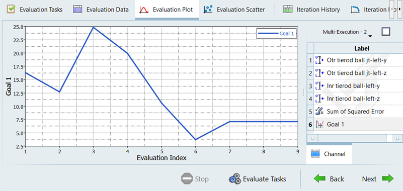
Figure 8. Optimization history plotIn this panel, you can see the plots variations in the values of the objectives, constraints, design variables, and responses during different design iterations. The Iteration History Table displays the same data in a tabular format.
Note that in this study, iteration 6 is the optimal configuration.
Save your study to <working directory> as Study_2.hstudy.
Step 2: Compare the Baseline and Optimized Models
-
Click the Page Layout icon,
 , on the toolbar and select the two-window layout.
-
Click the Build Plots icon,
 , on
the toolbar.
, on
the toolbar.
-
Plot another curve from the file.
<working directory>\approaches\opt_1\run__00006\m_1\m_1.abf using steps 11-14
You should end up with a session looking like the one shown below. Notice the optimized toe-curve.
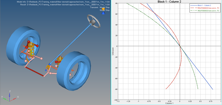
Figure 9. Optimization resultsYou may also overlay the animation of the optimal configuration (run 6) over the nominal run. Notice the toe angle differences.