Body: Flexible
Model ElementBody_Flexible defines a flexible body object in MotionSolve.
Description
- Linear flexible body: This is a representation of the flexible component obtained by carrying out a Component Mode Synthesis (CMS) analysis. This entity has mass and inertia properties just like a rigid body. In addition, it has flexibility properties that allow it to deform under loads. The deformation is defined using a set of spatial mode shapes and time dependent modal coordinates. Such a body is linearly flexible meaning that it cannot handle non-linear or "large" deformations.
- Non-linear Finite Element (NLFE) body: This is a fully non-linear finite element representation of the flexible component and does not require a pre-analysis to create. This entity, like the CMS flexible body, has mass and inertia properties. Owing to its fully non-linear formulation, this body is capable of handling "small" as well as "large" deformation.
A Body_Flexible may be connected to the rest of the system using any combination of constraints, motions, or applied forces. It does not support contact natively.
Linear Flexible Body
The CMS flexible body operates in 3D space where it can simultaneously undergo large overall motion and small deformations. Two types of CMS methods are supported: Craig-Bampton and Craig-Chang.
- General information about the number of modes selected, rigid body properties, number of interface nodes, and so on.
- Mode data block, which contains the frequency, eigenvalue, and damping for each mode.
- Node data block, which contains:
- Coordinates of the interface nodes chosen.
- Mode shape corresponding to each of the interface nodes selected.
- Inertia data block, which contains the inertia invariants required for the definition of the flexible body.
Every Body_Flexible element also refers to a Local Part Reference Frame (LPRF). This is the global coordinate system used for the finite element model and also serves as the coordinate system for the information in the Reference_FlexData element.
- Modal damping as a function expression, or
- DMPSUB user defined subroutine.
A finite element mesh and an optional scale factor may be provided while defining a Body_Flexible. This information is used to generate an H3D animation file. The H3D file containing the mesh data and the animation scale is not directly used in the simulation.
NLFE Body
- Define the grid locations and their gradients
- Define the elements and their types
- Define the properties of the flexible component
- Define any other connector elements
The formulation of the NLFE body is based on the "Absolute Nodal Coordinate Formulation" in which the coordinates are always defined with respect to the global frame. Thus this body does not refer to a Local Part Reference Frame (LPRF), unlike the CMS flexible body.
You may specify Rayleigh damping for your flexible component. This damping is numerical in nature and care should be taken while using this parameter. Too large a value may lead to solution instabilities.
The connectivity and geometric properties defined for the NLFE body in MotionView determine the mesh for visualization of the NLFE body in the post processor. The animation H3D can be used to visualize stresses, strains and displacements just like the CMS flexible body.
CMS Flexible Body Format
<Body_Flexible
      id                          = "integer"
      label                       = "string"
      lprf_id                     = "integer"
      mass                        = "real"
      inertia_xx                  = "real"
      inertia_yy                  = "real"
      inertia_zz                  = "real"
      inertia_xy                  = "real"
      inertia_yz                  = "real"
      inertia_xz                  = "real"
      cm_x                        = "real"
      cm_y                        = "real"
      cm_z                        = "real"
      h3d_file                    = "string"
      flexdata_id                 = "integer"
      animation_scale             = "real"
      is_user_damp                = "{ TRUE | FALSE }"
   {  cdamp_expr                  = "string"
     |usrsub_dll_name             = "string"
      usrsub_param_string         = "USER([par_1, ..., par_n])"
      usrsub_fnc_name             = "string"
     |script_name                 = "string"
      interpreter                 = "PYTHON"
      usrsub_param_string         = "USER([par_1, ..., par_n])"
      usrsub_fnc_name             = "string"
   }
[[
      rigidified                  = "{ TRUE | FALSE}"
      geostiff                    = "{ TRUE | FALSE}"
      v_ic_x                      = "real"
      v_ic_y                      = "real"
      v_ic_z                      = "real"
      w_ic_x                      = "real"
      w_ic_y                      = "real"
      w_ic_z                      = "real"
      v_ic_x_flag                 = "{ TRUE | FALSE}"
      v_ic_y_flag                 = "{ TRUE | FALSE}"
      v_ic_z_flag                 = "{ TRUE | FALSE}"
      w_ic_x_flag                 = "{ TRUE | FALSE}"
      w_ic_y_flag                 = "{ TRUE | FALSE}"
      w_ic_z_flag                 = "{ TRUE | FALSE}"
      vm_id                       = "integer"
      wm_id                       = "integer"
]]
/>
NLFE Body Format
<Body_Flexible
      id                          = "integer"
      label                       = "string"
      ref_marker_id               = "integer"
      ancf_file                   = "string"
      rayleigh_damping            = "real"
      num_i_marker                = "integer"
[[
      v_ic_x                      = "real"
      v_ic_y                      = "real"
      v_ic_z                      = "real"
      v_ic_x_flag                 = "real"
      v_ic_y_flag                 = "real"
      v_ic_z_flag                 = "real"
      w_ic_x                      = "real"
      w_ic_y                      = "real"
      w_ic_z                      = "real"
      w_ic_x_flag                 = "real"
      w_ic_y_flag                 = "real"
      w_ic_z_flag                 = "real"
]]
>
< ! -- The area below lists IDs of markers attached to the NLFE body-- >
ID1     ID2     ...     IDn
</Body_Flexible>
Attributes
- id
- Element identification number (integer>0).
This is a number that is unique among all Body_Flexible elements.
- label
- The name of the Body_Flexible element.
- lprf_id
- (CMS only) Specifies the ID of a Reference_Marker that defines the finite element global coordinate system in the MBS model.
- ref_marker_id
-
(NLFE only) Specifies the ID of a Reference_Marker. The components of the relative displacement, relative velocity and forces are resolved in the coordinate system specified by ref_marker_id.
This is set to the ground reference frame.
- mass
- (CMS only) Specifies the mass of the Body_Flexible object. For the CMS flexible body, the mass is computed using information available in the CMS H3D file that represents the flexible component.
- inertia_xx, inertia_yy, inertia_zz, inertia_xy, inertia_yz, inertia_xz
- (CMS only) Defines the moments of inertia and the products of inertia of the CMS flexible body
about the origin of the lprf_id marker and about its x-,
y- and z-axes, respectively.
The attributes inertia_xx, inertia_yy, inertia_zz, inertia_xy, inertia_yz, and inertia_xz are typically calculated using information that is available in the CMS flexibly body representation.
When specified, inertia_xx, inertia_yy, and inertia_zz need to be strictly positive.
- cm_x, cm_y, cm_z
- (CMS only) Center marker x, y and z.
- h3d_file
- (CMS only) Specifies the name of the file that contains all the nodes in the finite element mesh. This file is needed only for creating an animation file. The solver does not use it for analysis.
- ancf_file
- (NLFE only) Specifies the complete or relative path and name of the XML that contains geometric and material property data for the NLFE body
- flexdata_id
- (CMS only) Specifies the ID of the Reference_FlexData object that contains the CMS representation for the flexible body.
- animation_scale
- (CMS only) Specifies the scale factor for animating the mode shapes. This information is used only for creating the animation file. The solver does not require this for analysis.
- is_user_damp
- (CMS only) A Boolean value that specifies how the damping coefficient for each mode is
specified. A value of "TRUE" indicates that the damping is
specified using either an expression or a user defined subroutine.
A value of "FALSE" causes MotionSolve to ignore the damping expression or user defined subroutine data provided in the Body_Flexible element and instead, use the damping values specified in the Reference_FlexData element.
- cdamp_expr
- (CMS only) A state dependent expression that defines the damping coefficient for each mode. Any valid run-time MotionSolve expression can be provided as input. MotionSolve uses this parameter only when is_user_damp = "TRUE".
- usrsub_dll_name
- (CMS only) Specifies the path and name of the DLL or shared library containing the user subroutine. MotionSolve uses this information to load the subroutine specified by usrsub_fnc_name in the user library at run time. Use this keyword only when is_user_damp = "TRUE".
- usrsub_param_string
- (CMS only) The list of parameters that are passed from the data file to the user defined subroutine. Use this keyword only when type = USERSUB is selected. This attribute is common to all types of user subroutines/scripts.
- usrsub_fnc_name
- (CMS only) Specifies an alternative name for the user subroutine DMPSUB.
- script_name
- (CMS only) Specifies the path and name of the user written script that contains the routine specified by usrsub_fnc_name.
- interpreter
- (CMS only) Specifies the interpreted language that the user script is written in. Valid choices are MATLAB or PYTHON.
- rayleigh_damping
- (NLFE only) Specifies the value of a Rayleigh damping coefficient for the NLFE body. 1
- num_i_marker
- (NLFE only) Specifies the number of markers that are attached to this NLFE body. These markers
can be thought of as interface markers where the NLFE body can connect with
the rest of the multibody system.
num_i_marker > 0 1
- rigidified
- (CMS only) A Boolean flag that allows you to convert the flexible body to a rigid body. This flag is optional. The default value for this flag is rigidified = "FALSE". 4
- geostiff
- (CMS only) A Boolean flag that allows you to model the geometric stiffening effect in your CMS
flexible body. The default for geostiff is
"FALSE".Note: The geometric stiffening data must be available in the H3D for MotionSolve to be able to use it. See Comment 5 for more details.
- v_ic_x, v_ic_y, v_ic_z
- These attributes specify the initial translational velocity of the flexible body along the X, Y
and Z axes respectively.
For CMS flexible bodies, you may define the local part reference frame (LPRF) velocities with respect to any coordinate system. The marker representing this coordinate system is defined by vm_id.
For NLFE bodies, the velocities are applied along the global X, Y and Z directions respectively.
v_ic_x and v_ic_z are optional. They are assumed to be zero when not specified. MotionSolve may change these values to ensure that the initial velocities satisfy the system constraints.
- w_ic_x, w_ic_y, w_ic_z
- These attributes specify the initial angular velocity of the flexible body about the X, Y and Z
axes respectively.
For CMS flexible bodies, you may define the local part reference frame (LPRF) velocities with respect to any coordinate system. The marker representing this coordinate system is defined by wm_id.
For NLFE bodies, the velocities are applied about the global X, Y and Z axes, respectively.
w_ic_x, w_ic_y and w_ic_z are optional. They are assumed to be zero when not specified. MotionSolve may change these values to ensure that the initial velocities satisfy the system constraints.
- v_ic_x_flag, v_ic_y_flag, v_ic_z_flag
- Boolean flags that indicate whether the X, Y or Z velocity is known exactly or is just an
initial guess.
"TRUE" means this initial condition is applied exactly unless it is in conflict with a Motion input.
"FALSE" means this initial condition is applied as an initial guess. It may be changed by MotionSolve to ensure that all constraints are satisfied.
- w_ic_x_flag, w_ic_y_flag, w_ic_z_flag
- Boolean flags that indicate whether the angular velocities about the X, Y or Z axis is known
exactly or is just an initial guess.
"TRUE" means this initial condition is applied exactly unless it is in conflict with a Motion input.
"FALSE" means this initial condition is applied as an initial guess. It may be changed by MotionSolve to ensure that all constraints are satisfied.
- vm_id
- (CMS only) Specifies the ID of a marker with respect to which the translation initial velocities are applied. If not specified, the velocities are applied with respect to the global frame
- wm_id
- (CMS only) Specifies the ID of a marker with respect to which the rotational initial velocities are applied. If not specified, the velocities are applied with respect to the global frame
- ID1ID2… IDn
- (NLFE only) A list of the IDs of the markers that are used to connect the NLFE body to the rest of the multibody system
Example 1
The image below shows the boom in a back-hoe loader:
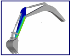
Figure 1. Using a CMS Flexible Body to Model the Boom in a Back-hoe Loader
Because of the large hydraulic forces acting on the arm, the flexibility of the arm plays a significant role in determining the overall behavior of the system and the forces at the pivot points.
The definition of the flexible boom is shown below. Note that is_user_damping is set to "FALSE" and hence, damping is defined in the Reference_FlexData element.
The flexible body refers to Reference_FlexData 11. This defines the CMS representation of the flexible body.
- The flexible body has 5 attachment points or interface nodes.
- 31 modes are used to represent the deformation shapes.
- The original finite element mesh has 36,382 nodes.
- The mass of the body is 343.79447 Kg.
- The inertia at zero deformation is:
- Ixx = 71.424 kgm2, Iyy = 204.970 kgm2, Izz = 270.996 kgm2
- Ixy = -108.571 kgm2, Iyz = -0.0007927 kgm2, Izx = -0.0013968 kgm2
- All modes above 1000 radians/second are critically damped (mode numbers 25 - 37).
The Reference_FlexData card is shown below.
<Reference_Flexdata
     id                  = "11"
     num_nodes           = "36382"
     num_sel_modes       = "31"
     num_sel_nodes       = "5" >
<ModeData>
<!--    ID       Frequency      Eigenvalue          Damping  -->
         7   1.6383385E+02   1.0596634E+06    1.0000000E-01
         8   2.1524734E+02   1.8290949E+06    1.0000000E-01
         9   2.3918134E+02   2.2584748E+06    1.0000000E-01
        ...
        34   2.6830053E+03   2.8418668E+08    1.0000000E+00
        35   2.7798731E+03   3.0507780E+08    1.0000000E+00
        36   3.5534390E+03   4.9849222E+08    1.0000000E+00
        37   4.4473195E+03   7.8083150E+08    1.0000000E+00
     </ModeData>
     <NodeData>
<!--    ID               X               Y               Z   -->
     320900  -4.1635098E+00  -3.7339999E-01  -1.3000000E-01
     320905  -3.7123201E+00   1.6183400E-01   1.0700000E-10
     320906  -4.2820601E+00   1.4321400E-01  -2.5000000E-02
     320917  -5.7897798E+00  -1.0092300E+00  -1.6000000E-01
     320919  -6.1077402E+00  -1.1671100E+00  -1.3000000E-01
<!-- Mode Shape -->
  -2.7620662E-03  -1.5999271E-02  -1.3520377E-02  -1.2305416E-01   2.1246834E-02  -1.8486151E-06
   2.3995511E-07  -2.7162932E-06  -8.7264590E-02  -3.7223276E-02   1.3226432E-01  -1.4547608E-05
  -2.7368159E-03  -3.5339149E-03  -1.4723917E-03  -1.4127485E-01   1.0950999E-01   1.5551852E-05
   ...
   1.5056358E-02   9.0596480E-03   6.5006730E-05  -2.5446518E-04   1.5557368E-03   1.5840490E-01
  -4.4426341E-02   1.0682830E-01   5.2728883E-05   2.6002291E-03  -1.4042209E-03  -4.8935637E+00
   1.8613113E-02  -4.1820321E-02   6.9122898E-06  -7.9896546E-04  -5.2661070E-04  -5.9843439E-01
     </NodeData>
     <InertiaData>
   8.7288856E-01  -4.8791962E-01  -4.4323963E-06   4.8791962E-01   8.7288856E-01  -4.7179542E-06
   6.1709705E-06   1.9555952E-06   1.0000000E+00  -4.8517495E+00  -5.0135241E-01  -2.1201009E-06
   2.6295942E+02   8.0369704E+00   2.6993996E+00   1.5783882E+02  -9.4482949E+02  -4.9331539E-03
  -9.4482949E+02   8.2977114E+03  -1.1581632E-03  -4.9331539E-03  -1.1581632E-03   8.4501514E+03
     </InertiaData>
  </Reference_Flexdata>
Example 2
In the following example, damping is specified using a MotionSolve expression. Note that is_user_damp is set to "TRUE".
<Body_Flexible
    id                = "30102"
    lprf_id           = "63330102"
    h3d_file          = "../../flex_h3d/beam.h3d"
    is_user_damp      = "TRUE"
    cdamp_expr        = "IF (FXFREQ-100:0.01,0.1,IF (FXFREQ-1000:0.1,1.,1))"
    flexdata_id       = "30102"
    animation_scale   = "1."
/>
Example 3
In the following example, damping is specified using a user defined subroutine (DMPSUB). Note that is_user_damp is set to "TRUE".
<Body_Flexible
    id                   = "30102"
    lprf_id              = "633301012"
    h3d_file             = "../../flex_h3d/beam.h3d"
    is_user_damp         = "TRUE"
    usrsub_param_string  = "USER (0.01,100,0.1,1000,1)"
    usrsub_dll_name      = "NULL"
    usrsub_fnc_name      = "DMPSUB"
    flexdata_id          = "30102"
    animation_scale      = "1."
/>
Example 4
The following lines show an example for converting a flexible body (0-3 seconds) to a rigid body (3-6 seconds) and then back to flexible body (6-10 seconds).
<Simulate
    analysis_type      = "Transient"
    end_time           = "3.0"
    print_interval     = "0.01"
/>
<Body_Flexible
    id                 = "30102"
    rigidified         = "TRUE"
/>
<Simulate
    analysis_type      = "Transient"
    end_time           = "6.0"
    print_interval     = "0.01"
/>
<Body_Flexible
    id                 = "30102"
    rigidified         = "FALSE"
/>
<Simulate
    analysis_type      = "Transient"
    end_time           = "10.0"
    print_interval     = "0.01"
/>
Example 5
The following example shows how an NLFE body can be used to model a stabilizer bar used in the front suspension of an automobile.
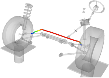
Figure 2. NLFE Body Used to Create a Stabilizer Bar Flexible Part
The NLFE body is represented in MotionSolve by the Body_Flexible statement:
<Body_Flexible
      id                          =   "30601"
      label                       =   "Stabilizer Bar"
      ref_marker_id               =   "30101010"
      ancf_file                   =   "stabar_NLFE_30601.xml"
      rayleigh_damping            =   "0.5"
      num_i_marker                =   "4">
30601011    30601191    30601091    30601111
</Body_Flexible>
Markers 30601011, 30601191, 30601091 and 30601111 are used to attach the NLFE system to the rest of the vehicle. Marker 30101010 is a ground reference marker located at the origin.
The NLFE body is defined in the file stabar_NLFE_30601.xml as follows:
<ANCF Model>
    <UNIT force="NEWTON" mass="KILOGRAM" length="MILLIMETER" time="SECOND"/>
    <GRID id="306001" x="1120.000000" y="-544.000000" z="989.000000" rx="0.000000 1.000000 0.000000" ry="-1.000000 0.000000 0.000000" rz="0.000000 -0.000000 1.000000"/>
    <GRID id="306002" x="1120.000000" y="-515.000000" z="989.000000" rx="0.948371 -0.279089 -0.150668" ry="0.282312 0.959323 -0.000000" rz=0.144539 -0.042535 0.988584"/>
    ...
    <GRID id="306018" x="1120.000000" y="515.000000" z="989.000000" rx="-0.286957 0.956858 0.045589 ry="-0.957854 -0.287255 -0.000000 rz="0.013096 -0.043667 0.998960"/>
    <GRID id="306019" x="1120.000000" y="544.000000" z="989.000000" rx="0.000000 1.000000 0.000000" ry="-1.000000 0.000000 0.000000" rz="0.000000 -0.000000 1.000000"/>
    <BEAMC id="20000" pid="10000" g1="306001" g2="306002"/>
    ...
    <BEAMC id="20017" pid="10000" g1="306018" g2="306019"/>
    <PBEAMC id="10000" mid="3000000" ri1="0.000000" ro1="10.000000" ri2="0.000000" ro2="10.000000" nf-"1" nx="5" nr="4" nt="10" ngx="5" ngr="4" ngt="12"/>
    <MAT1 id="3000000" e="210000" nu="0.3" rho="7.86e-006"/>
</ANCFModel>
As can be seen from the file above, the stabilizer bar is defined by BEAM elements of a circular cross section. The NLFE body refers to a linear elastic material.
Comments
- MotionSolve
supports two kinds of flexible bodies - CMS and NLFE flexible bodies. The
following table lists key comparisons between the two:
CMS flexible body NLFE flexible body Creating flexible bodies User meshing is required to represent the component No user meshing required for creating LD Body sub-systems through MotionView An additional CMS analysis is required to generate a modal representation of the flexible component No analysis required to create an LD body. The LD Body can be created and modified directly in MotionView Line, shell and solid elements are supported Only line elements are supported Connect to joints, forces etc. by defining interface nodes in CMS analysis All nodes can be used as interface nodes - no special handling is required. Modeling flexibility in components Only accurate up to a linear deformation range, that is, for small deformations; Must capture enough modal information to represent physical deformation accurately
Fully non-linear formulation allows accurate solution for small and large deformations without any reduction analysis Modeling geometric non-linearity in flexible components Cannot handle large deformations in general The BEAM and CABLE element allow you to model large deformations in your flexible components Modeling material non-linearity in flexible components Does not support non-linear material models You can model your flexible components with hyper elastic as well as linear elastic materials Recover stresses and strains Yes Yes. MotionSolve writes out a 3D representation of the beam and cable elements to enable stress, strain and displacement visualizations in HyperView - CMS Flexible Bodies
- CMS flexible bodies are created by performing a component mode
synthesis on an FE model using Altair's FE Solver OptiStruct. Both Craig-Bampton and
Craig_Chang methodologies are supported. The CMS data is stored
in a Reference_FlexData element and is
referred to by the attribute flexdata_id.
OptiStruct can accept finite
element data from the following sources.
- HyperMesh
- Patran
- Nastran
- Abaqus
- NLFE Bodies
- NLFE bodies are created within MotionView either individually or through
sub-systems. The NLFE body is defined by its geometric and
material properties. MotionSolve
currently supports LINE elements (i.e. elements that connect two
points in space). Two kind of elements are supported - CABLE and
BEAM elements. The table below lists key differences between the two:
Element Description CABLE The CABLE element does not resist shear or torsion forces. This implies that the cross section of this element does not change. This element can be used to model cables, wires etc.
BEAM The BEAM element resists all forms of deformation which implies that the cross section can also deform with load. This can be visualized in HyperView while using this element. Multiple cross sections are supported for the BEAM element:- Circular (solid and hollow)
- Rectangular or Box (solid and hollow)
- Channel
- Cross
- Hat
- H, I, L, T and Z sections
This element can be used to model beams, springs, belts, rubber components etc.
- MotionSolve
provides you with non-linear hyper-elastic material models to simulate
elastomers (for example rubber) and other materials that can undergo large,
reversible elastic deformations. On removal of the load, these materials return
to their original shape. Such materials typically have the following
characteristics:
- They can undergo large deformations and thus have large strain
- The relationship between the stress and strain is highly non-linear
often containing multiple inflection points
Shown below is a stress-strain relationship for a uniaxial test of a rod modeled using BEAM elements and using different hyper-elastic material models:
 Figure 3. Engineering Stress vs Engineering Strain for Hyper-elastic Material
ModelsThree non-linear hyper-elastic material models are available to use:
Figure 3. Engineering Stress vs Engineering Strain for Hyper-elastic Material
ModelsThree non-linear hyper-elastic material models are available to use:- Neo-Hookean compressible: This is the simplest form of a hyper-elastic material model and is based on a strain energy density function. The material Shear Modulus, Poisson's ratio and element density are specified as inputs for this model.
- Mooney-Rivlin: The MR material model is a development of the Neo-Hookean model and is available in a two-parameter form in MotionSolve. Such a model is useful when the material stress-strain curve has a single curvature i.e. no inflection points. The material's Poisson ratio and density, in addition to two material constants are specified as inputs for this model. The two material constants are typically obtained from curve fitting of test data obtained from axial or biaxial compression or tension tests.
- Yeoh: The Yeoh model within MotionSolve is available as a three parameter model that has been shown to satisfactorily model various modes of deformation based on data from a uniaxial tensile test. 6
- MotionSolve does not use Euler Angles to represent large rotations. Consequently, it does not suffer from the "Euler Singularity" problem, where the angles defining the 3D rotation are non-unique.
- The Boolean attribute
rigidified is used to specify whether the flexible body
should be modeled as such or as a rigid body. This can also be done using the
<Body_Flexible> command element (see example 4
below) or by using the MotionSolve specific utility
sub-routine c_modset.Note: A rigidified flexbody is computationally more efficient than a pure flexible body, but less efficient than a pure rigid body, due to implementation differences. As a result, in some cases where the solver takes many iterations to achieve a static equilibrium, it may be a good practice to do the following:
- Convert all flex-bodies to rigidified flex bodies.
- Run a static simulation.
- Convert all rigidified flex bodies back to pure flex bodies.
- Run a static simulation again.
The above steps may reduce the total number of solver steps required to achieve static equilibrium. However, since static convergence is model dependent, the above may not help in some cases.
- Geometric or stress stiffening is a non-linear
geometric effect most commonly seen in thin, slender structures (flexible
control arms, rotor blades, turbine blades, etc.) subjected to a tension load.
In such a case, the frequency of the fundamental modes increases as the tension
is increased. This effect can also be seen in a flexible beam undergoing large
rigid body rotation, for example a rotor blade. Due to increasing rotation
speed, the tensile (centrifugal) force acting on the blade increases, which
increases the frequency of the beam's fundamental modes, thereby resulting in an
increased bending stiffness of the beam.
To include this coupling effect for your CMS flexible body, you need to generate the additional stiffening data (represented as <GeoStiff> in MotionSolve) at the time of generating the CMS flexible body.
- Mac Donald Brian J. Practical Stress Analysis with Finite Elements. Dublin: Glasnevin Publishing, 2007. Print.