Force: State Equation
Model ElementForce_StateEqn is an abstract modeling element that combines the modeling capabilities of the Control_StateEqn and the Force_Vector_TwoBody model elements.
Description
The Force_StateEqn is used to apply a vector force (FX, FY, FZ, TX, TY and TZ) and thus must have exactly 6 outputs.
- A vector of inputs u
- A vector of dynamic states x defined through a set of differential equations
- A vector of outputs y defined by a set of algebraic equations. Since the Force_StateEqn is used to apply a vector force (FX, FY, FZ, TX, TY and TZ) the number of outputs is fixed at 6.
The image below illustrates the basic concept of a dynamic system.

Figure 1. Inputs, Outputs, and States for a dynamic system.
For such a dynamic system, the Force_StateEqn computes the state vector x, given u and applies the output y as a vector force between the two specified bodies.
As with the Control_StateEqn, two types of Force_StateEqn elements are available in MotionSolve.
- Linear Dynamical Systems: These are characterized by four matrices: A, B, C, and D. These are
related to the dynamical system in the following way: The four matrices A, B, C, D are all constant valued. The first equation defines the states. The second equation defines the outputs.
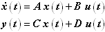
Figure 2.The A matrix is called the state matrix. It defines the characteristics of the system. If there are "n" states, then the A matrix has dimensions n x n. A is required to be non-singular.
The B matrix is called the input matrix. It defines how the inputs affect the states. If there are "m" inputs, the size the B matrix is n x m.The C matrix is called the output matrix. It defines how the states affect the outputs. If there are "p" outputs, the size the C matrix is p x n.
The D matrix is called the direct feed-through matrix. It defines how the inputs directly affect the outputs. The size the D matrix is p x m. - Nonlinear Dynamical Systems: These are characterized by two vector functions: F() and G(). These
are related to the dynamical system in the following way: The function F() returns the time derivative of x, when it is provided x(t) and u(t). The function G() returns the outputs y, when it is provided x(t) and u(t). Both F() and G() are required to be defined in user defined subroutines.
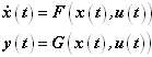
Figure 3.
Format
<Force_StateEqn
       id                      = "integer"
     [ label                   = "string" ]
       x_array_id              = "integer"
       ic_array_id             = { "integer"  | "0" }
     [ is_static_hold          = { "TRUE"  |  "FALSE" } ]
       i_marker_id             = "integer"
       j_floating_marker_id    = "integer"
       ref_marker_id           = "integer"
     [ u_array_id              = "integer" ]
    {
       type                    = "LINEAR"
           a_matrix_id         = "integer"
         [ b_matrix_id         = "integer" ]
         [ c_matrix_id         = "integer" ]
         [ d_matrix_id         = "integer" ]
     | type                    = "USERSUB"
           num_state           = "integer"
           usrsub_param_string = "USER( [[par_1][, ...][, par_n]] )"
           usrsub_dll_name     = "valid_path_name"
         [ usrsub_fnc_name     = "custom_fnc_name" ]
         [ usrsub_der1_name    = "custom_fnc_name" ]
         [ usrsub_der2_name    = "custom_fnc_name" ]
         [ usrsub_der3_name    = "custom_fnc_name" ]
         [ usrsub_der4_name    = "custom_fnc_name" ]
     | type                    = "USERSUB"
           num_state           = "integer"
           script_name         = valid_path_name
           interpreter         = "PYTHON" | "MATLAB"
           usrsub_param_string = "USER( [[par_1 [, ...][,par_n]] )"
         [ usrsub_fnc_name     = "custom_fnc_name" ]
         [ usrsub_der1_name    = "custom_fnc_name" ]
         [ usrsub_der2_name    = "custom_fnc_name" ]
         [ usrsub_der3_name    = "custom_fnc_name" ]
         [ usrsub_der4_name    = "custom_fnc_name" ]
>
   }
</Force_StateEqn>
Attributes
- id
- Element identification number (integer>0). This is a number that is unique among all Force_StateEqn elements.
- label
- The name of the Force_StateEqn element.
- is_static_hold
- A Boolean that specifies whether the values of the dynamic states, x, are kept fixed during
static equilibrium and quasi-static solutions.
- "TRUE"
- Implies that the dynamic states are kept constant during static and quasi-static solutions.
- "FALSE"
- Implies that the dynamic states are allowed to change during static equilibrium or quasi-static solutions.
- i_marker_id
- Specifies the Reference_Marker at which the force is applied. This is designated as the point of application of the force.
- j_floating_marker_id
- Specifies the Reference_Marker at which an equal and opposite reaction force is applied. This marker is moved around on the parent body so that it is always superimposed on i_marker_id. Such a construct allows Newton's third law to be automatically fulfilled. Note j_floating_marker_id may belong to rigid bodies or point masses only. They may not belong to flexible bodies.
- ref_marker_id
- Specifies the Reference_Marker whose coordinate system is used as the basis for defining the components of the force vector
- x_array_id
- Specifies the ID of the Reference_Array used to store the states "x" of this Force_StateEqn. You can use the ARYVAL() function with this ID to access the states in a MotionSolve expression. You can also use this ID in SYSFNC and SYSARY to access the state values from a user subroutine.
- u_array_id
- Specifies the ID of the Reference_Array used to store the inputs u of this Force_StateEqn. You can use the ARYVAL() function with this ID to access the states in a MotionSolve expression. You can also use this ID in SYSFNC and SYSARY to access the input values from a user subroutine.
- ic_array_id
- Specifies the ID of the Reference_Array used to store the initial values of the states, x of this Force_StateEqn. You can use the ARYVAL() function with this ID to access the states in a MotionSolve expression. You can also use this ID in SYSFNC and SYSARY to access the initial state values from a user subroutine.
- type
- Specifies the type of dynamic system being modeled. Select one from the choices
"LINEAR" or "USERSUB".
- "LINEAR"
- Specifies that the dynamic system being modeled is linear. The system definition is achieved by specifying the IDs of the A, B, C, and D matrices.
- "USERSUB"
- Specifies that the dynamic system being modeled is defined in user defined subroutines. The dynamic system can be linear or nonlinear.
- a_matrix_id
- Specifies the ID of the Reference_Matrix object containing the state matrix for a linear Force_StateEqn. The A matrix encapsulates the intrinsic properties of the dynamic system. For instance, the eigenvalues of A represent the eigenvalues of the system. Similarly, the eigenvectors of A represent the mode shapes of the dynamic system. A is a constant valued matrix. It is required to be invertible. If there are n states, the A matrix is of dimension n x n. Use only when type = "LINEAR".
- b_matrix_id
- Specifies the ID of the Reference_Matrix object containing the input matrix for a linear Force_StateEqn. The B matrix determines the contribution of the inputs u to the state equations.
- c_matrix_id
- Specifies the id of the Reference_Matrix object containing the output matrix for a linear Force_StateEqn. The C matrix determines the contribution of the states x to the outputs y. C is a constant valued matrix. If there are p outputs and n states, the C matrix is of dimension n x p.
- d_matrix_id
- Specifies the id of the Reference_Matrix object containing the feed-thru matrix for a linear Force_StateEqn. The D matrix determines the contribution of the inputs u to the outputs y. D is a constant valued matrix. If there are p outputs and m inputs, the D matrix is of dimension p x m.
- num_state
- An integer that specifies the number of states in the Force_StateEqn. num_state > 0.
- usrsub_param_string
- The list of parameters that are passed from the data file to the user defined subroutines YFOSUB, YFOXX, YFOXU, YFOYX and YFOYU. See Comment 4 for more explanation about these user defined subroutines. Use only when type = "USERSUB". This attribute is common to all types of user subroutines and scripts.
- usrsub_dll_name
- Specifies the path and name of the DLL or shared library containing the user subroutine. MotionSolve uses this information to load the user subroutines YFOSUB, YFOXX, YFOXU, YFOYX and YFOYU in the DLL at run time. Use only when type = "USERSUB".
- usrsub_fnc_name
- Specifies an alternative name for the user subroutine YFOSUB.
- usrsub_der1_name
- Specifies an alternative name for the user subroutine YFOXX.
- usrsub_der2_name
- Specifies an alternative name for the user subroutine YFOXU.
- usrsub_der3_name
- Specifies an alternative name for the user subroutine YFOYX.
- usrsub_der4_name
- Specifies an alternative name for the user subroutine YFOYU.
- script_name
- Specifies the path and name of the user written script that contains the routine specified by usrsub_fnc_name.
- interpreter
- Specifies the interpreted language that the user script is written in. Valid choices are MATLAB or PYTHON.
Example

Figure 4. Simple pendulum system
The model depicts a two dimensional problem. The system consists of a single mass that is fixed to a rigid, massless rod. The rod is attached to the ground via a revolute joint with rotation allowed about the global Y axis only. The mass of the spring bob is 1kg, and the length of the massless rod is 100mm. Gravity is applied in the negative Z direction. The angle between the rod and the global Z axis is denoted as and is measured in the model by the expression AZ(30101020,30102020).
- The pendulum mass is initially at rest. The initial angle is 90 degrees such that the pendulum is horizontal
- Due to gravity, the pendulum mass swings freely in the XZ plane, rotating about the global Y axis.
- The friction torque, Tf, counteracts the rotation of the pendulum at the hinge attachment, and consequently, the pendulum comes to rest after a while
The design parameters for the model are:
For this example, the Force_StateEqn element is:
<Force_StateEqn
     id                    = "301001"
     type                  = "USERSUB"
     x_array_id            = "535050504"
     y_array_id            = "535050508"
     u_array_id            = "535050505"
     num_state             = "2"
     num_output            = "6"
     usrsub_param_string   = "USER(1001,100.,0.31625,0.0004,1.,5.,1.5,1.25,0.5,0.3,0.)"
     usrsub_dll_name       = "ms_csubdll"
     usrsub_fnc_name       = "YFOSUB"
     is_static_hold        = "FALSE"
     i_marker_id           = "30101020"
     j_floating_marker_id  = "30102020"
     ref_marker_id         = "30102020"
  />
The I marker is defined as:
<Reference_Marker
     id                  = "30101020"
     label               = "Pivot-Marker I"
     body_id             = "30101"
     body_type           = "RigidBody"
     a00                 = "-1."
     a10                 = "0."
     a20                 = "0."
     a02                 = "0."
     a12                 = "1."
     a22                 = "0."
  />
The X, Y and U arrays are defined as:
<Reference_Array
     id                  = "535050504"
     type                = "X"
     num_element         = "2"
  />
  <Reference_Array
     id                  = "535050508"
     type                = "Y"
     num_element         = "6"
  />
  <Reference_Array
     id                  = "535050505"
     type                = "U"
     num_element         = "7"
     usrsub_param_string = "USER(1001,301001)"
     usrsub_dll_name     = "ms_csubdll"
     usrsub_fnc_name     = "ARYSUB"
  />
The U array contains seven values - the angular velocity of the pendulum, and the six joint reaction forces. This is made clearer by looking at the code for ARYSUB below.
The following is the code used for the user subroutines YFOSUB and ARYSUB:
DLLFUNC void STDCALL YFOSUB (int *id, double *time, double *par, int *npar,
                             int *dflag, int *iflag, int *nstate, double *states,
                             int *ninput, double *input, int *noutpt, double *stated,
                             double *output)
{
/*
#    YFOSUB evaluates the f and g in the following general state eqn
#           x' = f(x,u,t)
#           y  = g(x,u,t)
#    where x is the states, x' is the stated, u is the input, and y the output.
#    The output (y) is used as the force acting between the i and j markers.
*/
    if (int(par[0])==1001) // Joint Friction (Revolute)
    {
//      Parameter list for Joint Friction with Revolute Joints
//      (joint_id,sigma0,sigma1,sigma2,vS,Rb,Rp,Rf,muS,muD,Preload)
        double sigma0 = par[1];           // LuGre parameter
        double sigma1 = par[2];           // LuGre parameter
        double sigma2 = par[3];           // LuGre parameter
        double vS = par[4];               // Stribeck velocity
        double Rb = par[5];               // Bending arm
        double Rp = par[6];               // Pin Radius
        double Rf = par[7];               // Friction arm
        double muS = par[8];              // Static coefficient of Friction
        double muD = par[9];              // Dynamic coefficient of Friction
        double Preload = par[10];         // Friction Preload

        // Joint Reactions
        int i;
        double jReact[6];
        for(i=0;i<6;i++)
        {
            jReact[i] = input[i+1];
        }
        double Fr = pow((pow(jReact[0],2) + pow(jReact[1],2)),0.5);
        double Fa = jReact[2];
        double Fb = jReact[3]/Rb + jReact[4]/Rb;

        // Compute slip velocity

        double vSlipR = input[0]*Rp;
        double vSlipA = input[0]*Rf;

        // Compute Stribeck and Coulomb Force levels

        double FCr = muD;
        double FSr = muS;
        double FCa = muD;
        double FSa = muS;

        // GSE stuff

        double rExp = pow(2.718,(-pow((vSlipR/vS),2)));
        double aExp = pow(2.718,(-pow((vSlipA/vS),2)));

        double GVr = (FCr + (FSr - FCr)*rExp)/sigma0;
        double GVa = (FCa + (FSa - FCa)*aExp)/sigma0;

        stated[0] = vSlipR;
        stated[1] = vSlipA;
        if (fabs(GVr)>1e-12)
        {
            stated[0] -= states[0]*fabs(vSlipR)/GVr;
        }
        if (fabs(GVa)>1e-12)
        {
            stated[1] -= states[1]*fabs(vSlipA)/GVa;
        }

        // Friction Torque

        double FTrqR = (Fr+Fb+Preload)*Rp*(sigma0*states[0] + sigma1*stated[0] + sigma2*vSlipR);
        double FTrqA = (Fa)*Rf*(sigma0*states[1] + sigma1*stated[1] + sigma2*vSlipA);

        output[0] = 0.0;
        output[1] = 0.0;
        output[2] = 0.0;
        output[3] = 0.0;
        output[4] = 0.0;
        if (vSlipR<0)
        {
            output[5] = fabs(FTrqR + FTrqA);
        }
        else
        {
            output[5] = -fabs(FTrqR + FTrqA);
        }
    }
}
/*DLLFUNC void STDCALL ARYSUB (int *id, double *time, double *par,
int *npar, int *dflag, int *iflag, int *nvalue, double *value)
{
if (((int)par[0])==1001)
{
int errflg = 0;
int ipar[4];
int joint_id = (int)par[1];
int i_marker;
int j_marker;
char imark[80],jmark[80];
//Get the I and J marker ID for the joint
c_modfnc("Constraint_Joint",joint_id,"i_marker_id",imark,&errflg);
c_modfnc("Constraint_Joint",joint_id,"j_marker_id",jmark,&errflg);
i_marker = atoi(imark);
j_marker = atoi(jmark);
ipar[0] = i_marker;
ipar[1] = j_marker;
ipar[2] = j_marker;
//Query the solver for angular velocity using WZ(I, J, J)
c_sysfnc("WZ", ipar, 3, &value[0], &errflg);
ipar[0] = joint_id;
ipar[1] = 0;
ipar[2] = 2;
ipar[3] = j_marker;
//Get the Joint reaction forces - these will be used as input to the YFOSUB
c_sysfnc("JOINT", ipar, 4, &value[1], &errflg);
ipar[2] = 3;
c_sysfnc("JOINT", ipar, 4, &value[2], &errflg);
ipar[2] = 4;
c_sysfnc("JOINT", ipar, 4, &value[3], &errflg);
ipar[2] = 6;
c_sysfnc("JOINT", ipar, 4, &value[4], &errflg);
ipar[2] = 7;
c_sysfnc("JOINT", ipar, 4, &value[5], &errflg);
ipar[2] = 8;
c_sysfnc("JOINT", ipar, 4, &value[6], &errflg);
}
}
Figure 5. Comparison of angular displacement with and without friction in the revolute joint
Comments
- The Force_StateEqn element is equivalent to a combination of the Control_StateEqn (GSE component) model element and a Force_Vector_TwoBody (Force component) element. While the GSE component calculates the state and output vectors (given the input), the FORCE component applies the output from the GSE as forces and torques to the body specified by the i_marker_id and as reaction forces and reaction torques to the body specified by the j_floating_marker_id.
- As with the Control_StateEqn, the Force_StateEqn is also available in a "LINEAR" and "USERSUB" version. For more details on these, please refer to the documentation on Control_StateEqn.
- The "USERSUB" version of a
Force_StateEqn is more complex than most modeling elements
that are defined via user defined subroutines.
Five user subroutines may be needed. The first, YFOSUB is required. The other four, YFOXX, YFOXU, YFOYX, YFOYU, are required only when a stiff integrator (VSTIFF or MSTIFF) is used.
Name Inputs Outputs YFOSUB The states - x The inputs - u
The state derivatives, The outputs,
YFOXX The states - x The inputs - u
The matrix (n x n) of partial derivatives, YFOXU The states - x The inputs - u
The matrix (n x m) of partial derivatives, YFOYX The states - x The inputs - u
The matrix (p x n) of partial derivatives, YFOYU The states - x The inputs - u
The matrix (p x n) of partial derivatives, - The behavior of the dynamic states associated with a
Force_StateEqn element during static and quasi-static
solutions is governed by the attribute is_static_hold.
is_static_hold = "TRUE"
If the solution is done at time T=0, the states are kept fixed at the value specified by the IC array. If the solution is done following a dynamic simulation, then the value is kept fixed at the last value obtained from the dynamic simulation. The equations defining the states for the Force_StateEqn are replaced with the following:
x(t*) = x*, where x* is a constant.Note: When the dynamic states are kept fixed, their time derivatives are no longer zero at the end of the static equilibrium or a quasi-static step because the inputs u, which are typically time dependent, have changed. This may lead to transients if a dynamic solution were to be subsequently performed.is_static_hold = "FALSE"
The states are not kept constant, but allowed to change as the configuration of the entire system changes during the solution process. Here is how this is accomplished.
For static and quasi-static solutions, the derivative of the dynamic states is set to zero. This converts the GSE component of the Force_StateEqn to a set of algebraic equations.
The differential equations become:
(1) 
During the equilibrium solution, the inputs u change as the system changes its configuration to satisfy the equilibrium conditions. The above equations are solved to compute x for the current value of u.
This method ensures that the time derivative of the dynamic states is zero at the end of the static or quasi-static solution, and thus avoids introducing transients in a subsequent dynamic simulation.