Reference: Deformable Curve
Model ElementReference_DeformCurve specifies a deformable curve that is made to pass through the origins of a specified set of markers, using CUBIC spline interpolation. These markers may be on separate bodies. As the markers move in space, the curve shape is recalculated using CUBIC spline interpolation, thereby allowing the curve to deform.
Description
The curve can be opened or closed.
Format
<Reference_DeformCurve
     id               = "integer"
     u_span           = "real"
    [label            = "string"]
    [end_type_left    = "{NATURAL | PARABOLIC | PERIODIC | CANTILEVER}"]
    [lambda_left      = "real"]
    [end_type_right   = "{NATURAL | PARABOLIC | PERIODIC | CANTILEVER}"]
    [lambda_right     = "real"]
    [is_u_closed      = "boolean"]
     num_marker_id    = "integer">
           integer …      integer …        integer
  />
Attributes
- id
- Specifies the element identification number, (integer>0). This number should be unique among all Reference_DeformCurve elements.
- label
- An optional character string that defines a name for the modeling element.
- u_span
- Real value that defines the span of the u parameter. The u parameter goes from -u_span/2 to u_span/2. u_span > 0.
- end_type_left
-
Select one from NATURAL, PARABOLIC, PERIODIC, or CANTILEVER. 3
Default = NATURAL
- lambda_left
- A real valued parameter in the interval [0,1] that controls the left end condition for CUBIC spline interpolation. A value of 0 implies NATURAL end condition, while a value of 1 implies PARABOLIC end condition. This parameter is only applicable for the CANTILEVER type end condition.
- end_type_right
- Select one from NATURAL, PARABOLIC, and PERIODIC. 3
- lambda_right
- A real valued parameter in the interval [0,1] that controls the left end condition for CUBIC spline interpolation. A value of 0 implies NATURAL end condition, while a value of 1 implies PARABOLIC end condition. This parameter is only applicable for CANTILEVER type end condition.
- is_u_closed
- A Boolean value (TRUE or FALSE) that determines whether the markers that define the curves are closed or not. 5
- num_marker_id
- Number of markers whose origins lie on the curve. 6
Example 1
The following example demonstrates the use of the Constraint_PTdCV element, along with the Reference_DeformCurve and Post_Graphic elements.
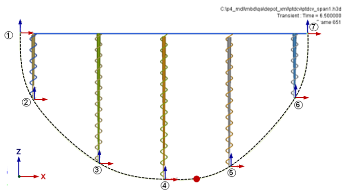
Figure 1. Using a Reference_DeformCurve to define a Constraint_PTdCV element
Figure 1 shows five slender bar-shaped rigid bodies constrained to a ground body, represented by the blue horizontal bar graphic, by translational joints with axes along the Z-direction. The bodies are connected to ground by linear spring-dampers. A deformable curve is defined to pass through seven markers (1-7 shown in the figure). Five of these markers, 2-6, are located at the lower tips of the rigid bodies. Two of these markers, 1 and 7, are located at either end of the ground body.
The curve is open, so is_u_closed is not specified, that is, it defaults to FALSE. The deformable curve, shown as a black dashed curve in Figure 1 is defined using the Reference_DeformCurve element as follows:
<Reference_DeformCurve
    id                  = "1"
    end_type_left       = "NATURAL"
    end_type_right      = "NATURAL"
    num_marker_id       = "7">
    1  2  3  4  5  6  7
 </Reference_DeformCurve>
The curve can be displayed in a post-processor such as HyperView by using a Post_Graphic element as shown below. In this example, 100 segments are used to approximate the cubic spline in the display window.
<Post_Graphic
    id                  = "500000"
    type                = "DeformCurve"
    curve_id            = "1"
    nseg                = "100"
 />
A small spherical body, shown as a red sphere, is constrained to slide along the deformable curve. This constraint is described by a Constraint_PTdCV as follows:
<Constraint_PTdCV
   id                  = "1"
   i_marker_id         = "30107060"
   ref_dcurve_id       = "1"
/>
The red sphere is given an initial velocity that causes it to slide on the deformable curve. As the sphere slides along the curve, the weight of the red sphere causes varying amounts of deflection to occur in each in each of the springs. The curve changes its shapes as a consequence. A dynamic analysis of this system will show the changing shape of the deformable curve, as the sphere slides back and forth because of gravity.
Example 2
This example demonstrates the use of the Constraint_PTdCV element for a closed curve, along with the Reference_DeformCurve and Post_Graphic elements.
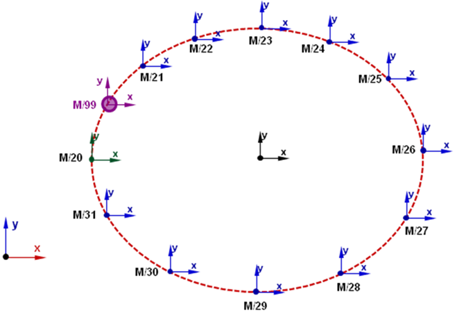
Figure 2. Defining a Closed, Deformable Parametric Curve
Referring to Figure 2 above, the closed curve is an elliptical shape that is defined by the origins of markers 20-31. Markers 20-31 belong to different bodies. Thus, their motion is governed by the motion of their underlying bodies. The MotionSolve input for this curve is shown below. Notice that since the curve is closed, the first and last markers in the markers list are the same. This is emphasized by highlighting in red below.
<Reference_DeformCurve
       id               = "301"
       label            = "DeformableCurve 1"
       end_type_left    = "NATURAL"
       end_type_right   = "NATURAL"
       u_span           = "1."
       is_u_closed      = "TRUE"
       num_marker_id    = "13">
       20  21  22  23  24  25  26  27  28  29  30  31  20
</Reference_DeformCurve> - { x(-0.5) y(-0.5) z(-0.5) } = { x(0.5) y(0.5) z(0.5) }.
- { x''(-0.5) y''(-0.5) z''(-0.5) } = { x''(0.5) y''(0.5) z''(0.5) }
A small spherical body, shown as a purple sphere in Figure 2 is constrained to slide along the deformable curve. The center-of-mass of the sphere is defined by Marker 99. This constraint is described by a Constraint_PTdCV as follows:
<Constraint_PTdCV
     id                  = "1"
     label               = "Advanced Joint 0"
     i_marker_id         = "99"
     ref_dcurve_id       = "301"
  />
An initial velocity, vo, starts the sliding motion of the purple spherical body. Over time, because the bodies containing markers 20-31 can move in their own way, the initially circular shape will become non-circular.
The curve shape can be displayed in a post-processor such as HyperView by using a Post_Graphic element as shown below. In this example, 150 segments are used to approximate the curve shape in the display window.
<Post_Graphic
     id                  = "2"
     type                = "DeformCurve"
     curve_id            = "30"
     nseg                = "150"
/>
Comments
- Reference_DeformCurve is quite similar to
Reference_ParamCurve, except it can deform. The shape of the curve is
defined by the cubic spline that passes through the instantaneous origins of a set of
markers, shown in Figure 3 below
with brick-red spheres. Reference_DeformCurve is therefore a
parametric, deformable curve in 3D space. u is a free curve parameter that defines the
extent of the curve. It can vary from umin = - u_span/2
to umax = + u_span/2. Referring to Figure 3, the coordinates of any arbitrary P point on the curve, as measured in OXYZ, can be represented uniquely in terms of the free parameter u with three cubic-spline functions f(u), g(u) and h(u) that define the x-, y- and z-coordinates of P.
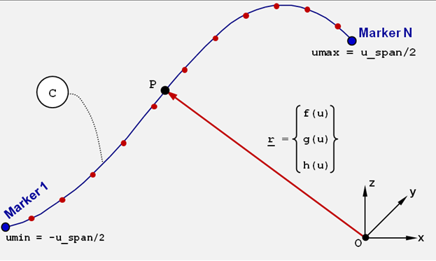
Figure 3. The Definition of a Reference_DeformCurve - Reference_DeformCurve can be opened or
closed. A closed curve has the property:
- { x(umin) y(umin) z(umin) } = { x(umax) y(umax) z(umax) }
- Reference_DeformCurve uses a CUBIC spline
interpolation which requires assumptions on the second derivative of the interpolating
function at the ends of the curve. The keywords NATURAL, PARABOLIC, PERIODIC and
CANTILEVER represent the four standard assumptions defined as follows:
- NATURAL (or free):
- PARABOLIC:
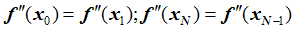
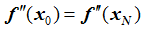
- PERIODIC:
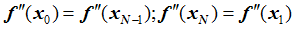
- CANTILEVER:

- Note that λ = 0.0 implies NATURAL (or free) end conditions and λ = 1.0 implies PARABOLIC end conditions.
- NATURAL (or free):
- The Reference_DeformCurve element does not possess any inherent inertia, stiffness, or damping properties.
- Closed curves are supported in MotionSolve. To define a closed curve, you must ensure that the first and last markers in the marker list that define the curve are the same. This will ensure the continuity of the curve. To obtain smooth, closed curves, do not specify end_type_left and end_type_right. Both will default to NATURAL. This guarantees the necessary smoothness.
- The minimum number of markers required to define an open curve is three due to the cubic nature of spline interpolation. For a closed curve, at least four markers are required (three markers for cubic spline interpolation and the fourth marker must be the same as the first to ensure smoothness of first and second derivatives).
- Deformable curves are used to define the Constraint_PTDCV, which constrains a point on a body to slide along the deformable curve.
- Occasionally, for an open deformable curve, you will see a
message, "Parameter U='value' goes out of intended range". This condition
occurs because the numerical methods have no obvious way to enforce the
limit:- u_span/2 ≤ u ≤ + u_span/2. In such a
situation, MotionSolve holds the "U" value at the boundary
(-u_span/2 or
+u_span/2) and continues with the simulation until
the point falls back in range, for example, - u_span/2 ≤ U ≤ +
u_span/2. If the model is well-defined, the point will fall back in
range. Note: If you see such a message in your simulation, please check the results carefully as they may be wrong, even though the simulation completes successfully.There are, however, modeling changes that you can make to minimize the occurrence of such a condition. Referring to Figure 3, one approach to handle this condition is to define two impact forces:
- Between marker P and marker 1
- Between marker P and marker N
When P tries to go beyond the limits specified for u, an impact force that pushes the marker P into the allowable range is generated.