Exercise 2: Nonlinear Gap Analysis
Create a Load Collector Defining Parameters
-
The error tolerances EPSU, EPSP, and EPSW can be left at their default
values.
For details on these tolerances, read the section Nonlinear Quasi-static Gap and Contact Analysis in the online help.
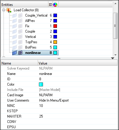
Figure 1.
Update the Load Steps
-
In the Select Loadcol dialog, select the nonlinear load
collector and click OK.
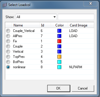
Figure 2.
Submit the Job
-
From the Analysis page, click the OptiStruct
panel.
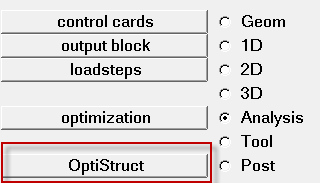
Figure 3. Accessing the OptiStruct Panel
The default files written to the directory are:
- rib_nonlinear.html
- HTML report of the analysis, providing a summary of the problem formulation and the analysis results.
- rib_nonlinear.out
- OptiStruct output file containing specific information on the file setup, the setup of your optimization problem, estimates for the amount of RAM and disk space required for the run, information for each of the optimization iterations, and compute time information. Review this file for warnings and errors.
- rib_nonlinear.h3d
- HyperView binary results file.
- rib_nonlinear.res
- HyperMesh binary results file.
- rib_nonlinear.stat
- Summary, providing CPU information for each step during analysis process.
Post-process the Results
-
Click the Curves Attributes icon
 and hide all components except the Web component.
- Activate the Auto apply mode check box
- Click on the components to turn off in the modeling window
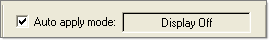
Figure 4. -
Go to the Contour panel
 .
.
-
Above the Results Browser in the left hand panel are the
Load Case and Simulation Selection drop-down menus. Select Subcase 1
(Coup_Vert) from the Load Case drop-down menu.
Figure 5. -
Click the XY Top Plane View icon
 to display a top view
of the Web.
to display a top view
of the Web.
-
Click Apply.
This should show the contour of stresses on the Web component under the coupled loading.
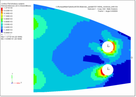
Figure 6. Stress Results on the Web From Nonlinear Gap Analysis -
Click Delete Page
 to end the HyperView session.