Structural Fluid-Structure Interaction Analysis
OptiStruct and AcuSolve are fully-integrated to perform a coupled Fluid-Structure Interaction Analysis based on a partitioned staggered approach.

Figure 1. Direct-Coupled Fluid-Structure Interaction (DC-FSI) Cycle
Input/Output
The detailed interface-specific input information is available in the Fluid-Structure Interaction page. Here you will look at solution-specific information required to run Structural FSI.
First look at the input data required from the OptiStruct side to set up the model. Subsequently, some information about the interface boundary conditions that are specific to Structural FSI is explained and to learn how to set them in the AcuSolve input file.
OptiStruct
Structural FSI is the coupled simulation of Nonlinear Direct Transient Analysis on the structure in conjunction with dynamic fluid flow analysis in the fluid domain.
- The initial time step (DT on NLPARM or TSTEPNL) should be set equal to the initial time step in the AcuSolve model. Fixed time step will be enforced throughout the solution and this will also be equal to the initial time step (adaptive time stepping is not supported).
- The FSI Bulk Data Entry should be added to the model. You can adjust the convergence tolerance parameters relevant to Structural FSI (FCNVTOL and DCNVTOL), the wait time (WAITTIME), and other parameters on this entry.
- The FSI Subcase Information Entry should be added to the nonlinear direct transient subcase and this entry should reference the corresponding FSI Bulk Data Entry.
The above steps allow you to successfully prepare the Nonlinear Transient Model for FSI analysis.
AcuSolve
Structural FSI is a coupling between the structural solver and the dynamic fluid flow analysis capabilities of the fluid solver. Therefore, you can look at the AcuSolve Command Reference Manual for detailed information about how to set up a model for dynamic fluid flow solutions. The deformations of the structural interface may lead to changes in fluid flow that affects the subsequent solution. Here a few parameters relevant to Structural FSI in the AcuSolve input file are looked at.
Use the EXTERNAL_CODE_SURFACE command to define the interaction between the
fluid interface and the corresponding parameters. The command specifies the surface
topology, as well as the interface proprieties.
EXTERNAL_CODE_SURFACE( "<structure_label>" ) {
    surfaces                            = Read( "<filename>.ebc" )
    shape                               = "<element type>"
    element_set                         = "<element set ID>"
    velocity_type                       = <wall/slip>
    mesh_displacement_type              = <tied/slip>
    gap_factor                          = <Real>
    gap                                 = <Real>
}
For Structural FSI, the velocity_type and
mesh_displacement_type define how the fluid and structural
interfaces interact (boundary conditions). The mesh_displacement
parameter defines whether the fluid mesh is tied to the solid mesh or allowed to
slip against the solid mesh surface. Set the
mesh_displacement_type=tied to tie the fluid
mesh to the solid mesh, or
mesh_displacement_type=slip to allow the fluid
mesh to slide against the solid surface, which acts as a guide surface. For
Structural FSI, there is exchange of displacements and pressure at the interface and
in addition, mesh displacement and velocity boundary conditions are present.
Therefore, the mesh parameter should be set to Arbitrary
Lagrangian Eulerian. For more information, refer to External Equation Field Settings of the Fluid Structure
Interaction page.
The velocity_type specifies how the fluid velocity behaves in relation to the
structural mesh velocity. Set velocity_type=wall
to tie the fluid velocity to the mesh velocity, or set
velocity_type=slip for the normal component of
the fluid velocity to be tied to the solid mesh velocity.
mesh_displacement and velocity_type
parameters. These are summarized in Table 1.
| Fluid-Solid Interface Conditions | Mesh Displacement | ||
|---|---|---|---|
| Tied | Slip | ||
| Velocity | Wall | Mesh Displacement:
|
Mesh Displacement:
|
| Velocity:
|
Velocity:
|
||
| Slip | Mesh Displacement:
|
Mesh Displacement:
|
|
| Velocity:
|
Velocity:
|
||
- Normal unit vector at the interface.
- Translational unit vector at the interface.
velocity=slip condition, the
velocity in translational direction is not constrained at the interface.When the fluid is allowed to slide along the solid mesh, neighborhood searches between the fluid
and solid meshes are continuously performed. The gap_factor
parameter specifies a non-dimensional (with respect to the length of the element
face) maximum allowable gap and the gap parameter specifies a non-dimensional
maximum gap distance between each quadrature point of the AcuSolve surface to the closest surface given by OptiStruct to check for gaps. If the distance is greater than
the gap, the computation stops with an error message.
Output
The FSI results are output to the corresponding working directories. The structural (OptiStruct) results are output to the H3D file by default and can be post-processed in HyperView. However, this file will not contain the fluid results. The fluid results are available in the AcuSolve .log file in the AcuSolve working directory. The AcuSolve .log file can also be loaded into HyperView.
For Structural FSI, currently, the fluid and structural results may be imported into a single HyperView session by choosing the overlay option. Only results common to both the structural and fluid analyses are available to be post-processed simultaneously.
The structural solution can be viewed in HyperView by opening the H3D file as illustrated in Figure 2.
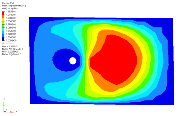
Figure 2. Fluid Domain FSI Results for the Enclosing Fluid Volume . (fluid results are overlaid on top of the existing Structural results)