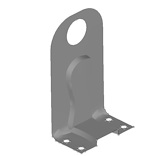
The objective of autobead is to offer automation of bead interpretation so that a
prototype-like design could be created automatically. Figure 1. L-bracket Layout
Launch HyperMesh and Set the OptiStruct User Profile
Launch HyperMesh.
The User Profile dialog opens.
Select OptiStruct and click
OK.
This loads the user profile. It includes the appropriate template, macro
menu, and import reader, paring down the functionality of HyperMesh to what is relevant for generating models for
OptiStruct.
Import the Model
Click File > Import > Solver Deck.
An Import tab is added to your tab menu.
For the File type, select OptiStruct.
Select the Files icon .
A Select OptiStruct file browser
opens.
Select the Lbkttopog_bead.fem file you saved
to your working directory. Refer to Access the Model Files.
Click Open.
Click Import, then click Close to
close the Import tab.
Run the Optimization
From the Analysis page, click OptiStruct.
Click save as.
In the Save As dialog, specify location to write the
OptiStruct model file and enter
Lbkttopog_bead for filename.
For OptiStruct input decks,
.fem is the recommended extension.
Click Save.
The input file field displays the filename and location specified in the
Save As dialog.
Set the export options toggle to all.
Set the run options toggle to optimization.
Set the memory options toggle to memory default.
Click OptiStruct to run the optimization.
The following message appears in the window at the completion of the
job:
OPTIMIZATION HAS CONVERGED.
FEASIBLE DESIGN (ALL CONSTRAINTS SATISFIED).
OptiStruct also reports error messages if any exist. The
file Lbkttopog_bead.out can be opened in a
text editor to find details regarding any errors. This file is written to the
same directory as the .fem file.
Click Close.
View the Results
Shape contour information is output from OptiStruct for all iterations. In addition,
Eigenvector results are output for the first and last iteration by default.
This section describes how to view those results in HyperView.
Review a Transient Animation of Shape Contour Changes
From the OptiStruct panel, click HyperView.
Load the results session.
From the menu bar, click File > Open > Session.
In the Open Session File dialog, navigate to your
working directory and open the Lbkttopog_bead.mvw file.
On the Animation toolbar, set the animation mode to (Transient).
Click to start the animation.
The animation shows how the shape changes over the course of the
optimization.
To slow down the animation, move the animation controls slider under the
Current Frame Indicator and adjust the Max Frame Rate slider.
Figure 2.
Review the Optimized Frequency Difference
In the top, right of the application, click to proceed to the next page.
On the Animation toolbar, set the animation mode to (Modal).
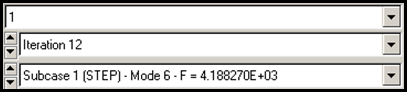
In the Results Browser, from the list of load cases, toggle
between Iteration 0 and Iteration 12.
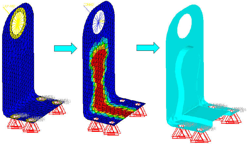
Figure 3.
The topography optimization yields an almost 100% increase in the
frequency of the first mode by reviewing the Mode 1-F value in the Simulation
list.
Click to animate the model.
Generate a New Model Based on a Topography Result
Apply Optimized Topography
Go back to HyperMesh.
Click return to exit the OptiStruct panel.
From the Post page, click the apply results panel.
Click simulation = and select DESIGN - ITER
12.
Click data type = and select Shape
Change.
Select displacements.
Set component selection to total disp.
Click nodes > all.
In the mult = field, enter 1.0.
Click apply.
The final nodal positions are applied to the structure.
Tip: Be careful with saving the model now, the HyperMesh database has changed. This model can be
used for further analyses. Results can now be viewed on the final
shape.
Click reject to get back the original shape.
Click return to go back to main menu.
Import Final Geometry using OSSmooth and Autobead
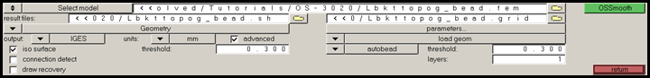
From the Post page, click the OSSmooth
panel.
Figure 4.
In the file: field, select the OptiStruct base input file from
which to extract the final geometry.
In the output: field, select the IGES output
format of the final geometry.
The default output format is STL. Other format
options are: Mview, Nastran, IGES, and H3D.
If you select IGES as the output format, select the output unit
type. The default is mm (millimeters).
Select load geom to load the new
geometry into the current HyperMesh session.
Select autobead, and enter
0.3 for the bead
threshold.
Leave the rest of the options at their default settings.
Click OSSmooth.
Click Yes to overwrite.
The new geometry will be automatically loaded into the
existing HyperMesh file,
turn off the display of all the elements to view the
new concept geometry.
OSSmooth can automatically create geometry based on the
new mesh.
Click FE > Surf to generate new geometry from the
optimization results.
Click Save and
Exit to continue.
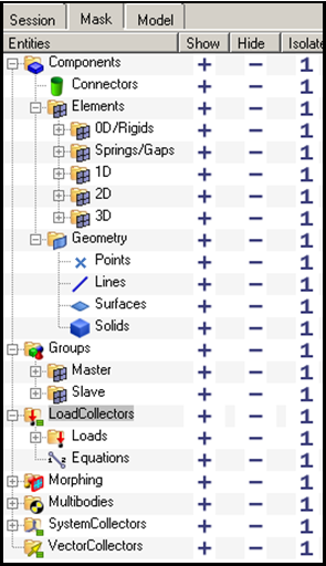
In the Mask Browser, click Isolate for
Geometry and click Hide for Load
Collectors.
Figure 5.
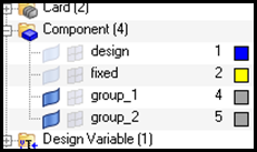
In the Model Browser, uncheck geometry
display for the original components design and fixed.
Figure 6.
New geometry for the optimized part is displayed. Figure 7.
 .
A Select OptiStruct file browser opens.
.
A Select OptiStruct file browser opens. (Transient).
 to start the animation.
The animation shows how the shape changes over the course of the optimization.
to start the animation.
The animation shows how the shape changes over the course of the optimization.
 to proceed to the next page.
 (Modal).