OS-T: 1371 Brake Squeal Analysis of Brake Assembly

In this tutorial you will perform a brake squeal analysis on a brake assembly. Disc brakes are operated by applying a clamping load using a set of brake pads on the disc. The friction generated between the pads and the disc causes deceleration, and can potentially induce a dynamic instability of the system. This phenomena is known as brake squeal.

For this model OptiStruct will predict an unstable mode and the instability is seen to occur at the point of mode coalescence, i.e., a pair of modes occur at the same frequency (mode coupling), and one of them is unstable. The unstable mode can be identified during complex eigenvalue extraction because the real part of the eigenvalue corresponding to an unstable mode is positive.

You can further design brake system which can be stabilized by changing the shape of the brake pads or material properties of the brake components to decouple the modes (which is not shown in this tutorial). The purpose of this tutorial is to conduct brake squeal analysis and identify the unstable modes (if they exist).

os1371_model
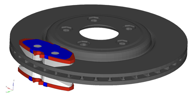
Figure 1. Model Review
brsq.fem File Data
  • Hexahedral Mesh is created for the brake assembly
  • All parts are defined with material MAT1
  • All parts are defined with Solid Element Property
  • A cylindrical coordinate system is defined with respect to the disc
  • S2S Contacts are defined between brake pad and disc
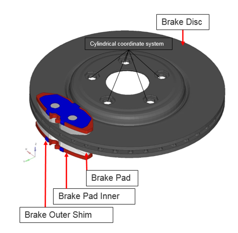
Two sub-cases are defined:

os1371_brake_assembly
Figure 2.
  1. Sub-case CLAMPLOAD: Nonlinear static analysis
    Pressure Load on Insulator (Inner and Outer), with SPC (DOF1).
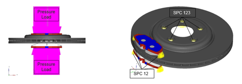
    os1371_dof1
    Figure 3.
  2. Sub-case ROTOR: Nonlinear static analysis with CNTNLSUB.
    Pressure Load on Pad and Rotation of the Disc, with non-zero SPC (DOF2).
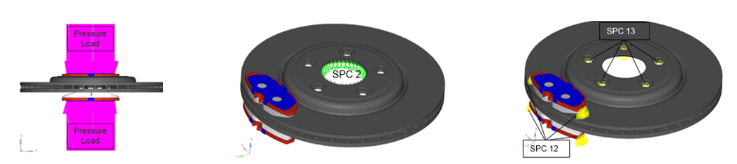
    os1371_dof2
    Figure 4.
    Tip:
    1. The prescribed rotation should be large enough to ensure the contact between the disc and the pad is in kinetic friction, but small enough to ensure small displacement NLSTAT.
    2. Kinetic friction is a constant value (independent of velocity), hence prescribing rotation using SPCD is equivalent to prescribing rotational speed. The important outcome is that the contact nodes are in kinetic friction mode and it does not matter how fast or how far you move this using SPCD.

Launch HyperMesh and Set the OptiStruct User Profile

  1. Launch HyperMesh.
    The User Profile dialog opens.
  2. Select OptiStruct and click OK.
    This loads the user profile. It includes the appropriate template, macro menu, and import reader, paring down the functionality of HyperMesh to what is relevant for generating models for OptiStruct.

Import the Model

  1. Click File > Import > Solver Deck.
    An Import tab is added to your tab menu.
  2. For the File type, select OptiStruct.
  3. Select the Files icon files_panel.
    A Select OptiStruct file browser opens.
  4. Select the brsq.fem file you saved to your working directory. Refer to Access the Model Files.
  5. Click Open.
  6. Click Import, then click Close to close the Import tab.

Set Up the Model

Create EIGRL and EIGC Cards

In this step, a modal method is used to solve the complex eigenvalue problem, which is more computationally efficient compared to extracting the complex modes directly. With this approach, first, the real modes are calculated via a normal modes analysis. Then, a complex eigenvalue problem is formed on the projected subspace spanned by the real modes which is much smaller than the real space. Here, both EIGRL and EIGC cards need to be defined.
  1. In the Model Browser, right-click and select Create > Load Collector.
  2. In the Name field, enter modal_space.
  3. Click Color and select a color from the color palette.
  4. Click Card Image and select EIGRL from the drop-down menu.
  5. Click V2 and input 5000.
    5000 is defined as the highest frequency bond.
  6. Click ND and input 100.
    100 real modes are required to produce the reduced space for complex eigenvalue analysis.
  7. Create another load collector named ceig_squeal.
  8. Click Card Image, and select EIGC.
  9. Click NORM and select MAX.
    MAX option will be used to normalize the eigenvectors.
  10. Click ND0 and input 55.
    The desired number of roots to be extracted is 55.

Define Load Step for Modal Complex Eigenvalue Analysis

  1. In the Model Browser, right-click and select Create > Load Step.
  2. In the Name field, enter BRSQ.
  3. Click Analysis type and select Complex eigen (modal) from the drop-down menu.
  4. For SPC, select DOF2 from the list of load collectors.
  5. For CMETHOD, select ceig_squeal_ from the list of load collectors.
  6. For METHOD(STRUCT), select modal_space from the list of load collectors.
  7. For STATSUB (BRAKE), select Sub-case ROTOR (ID 2).
    Tip: Create STATSUB (BRAKE) manually if this is not yet supported in HyperMesh.

Submit the Job

  1. From the Analysis page, click the OptiStruct panel.

    OS_1000_13_17
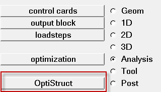
    Figure 5. Accessing the OptiStruct Panel
  2. Click save as.
  3. In the Save As dialog, specify location to write the OptiStruct model file and enter brsq for filename.
    For OptiStruct input decks, .fem is the recommended extension.
  4. Click Save.
    The input file field displays the filename and location specified in the Save As dialog.
  5. Set the export options toggle to all.
  6. Set the run options toggle to analysis.
  7. Set the memory options toggle to memory default.
  8. Click OptiStruct to launch the OptiStruct job.
If the job is successful, new results files should be in the directory where the brsq.fem was written. The brsq.out file is a good place to look for error messages that could help debug the input deck if any errors are present.

View the Results

Complex eigenvalue analysis computes the complex modes of the structure. The eigenvalues of the complex modes can be found in the brsq.out file. The complex eigenvectors can be reviewed in HyperView.
  1. Load the brsq.out file in a text editor.
    The complex modes contain the imaginary part, which represents the cyclic frequency, and the real part which represents the damping of the mode. If the real part is negative, then the mode is said to be stable. If the real part is positive, then the mode is unstable. The eigenvalues of the complex modes are shown below:
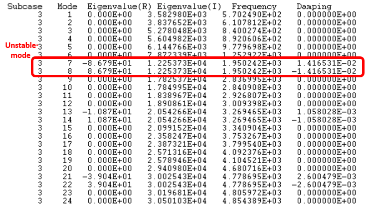
    os1371_results
    Figure 6.
  2. Load the brsq.h3d file into HyperView to review complex eigenvectors.
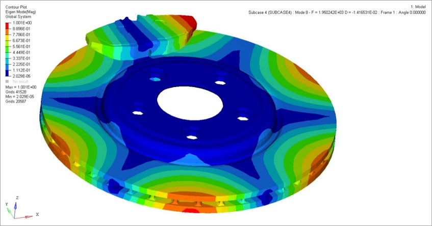
    os1371_results_hv
    Figure 7.