OS-V: 0820 Marlow Hyperelastic with Viscoelasticity Material Model

The combination of hyperelastic material models with viscoelasticity allows to model the strain rate dependent large strain response.

The Marlow model differs from most hyperelastic models by the concept not to use a small number of model parameters, but a scalar function to define the mechanical properties. It can be defined conveniently by providing the stress–stretch (stretch = engineering strain+1) curve without needs for parameter calibration. The coupling of the Marlow model and viscoelasticity is an approach to create a strain rate-dependent hyperelastic model which has good accuracy and is convenient to use. In this combination, the Marlow model requires to specify the stress–stretch curve for the instantaneous or long-term material response, while experimental data can be obtained only at finite strain rates.

Benchmark Model


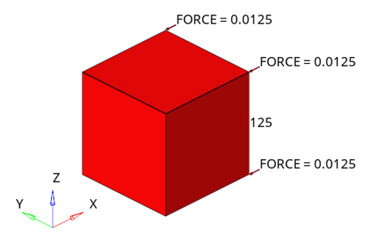
Figure 1. Benchmark FEM model with loads

The single CHEXA8 element model has an edge length of 1.0 mm. The Marlow model is derived from experimental data only using a single set of data. The test data in the form of uniaxial tension, uniaxial compression, equi-biaxial, or planar test is used. Deviatoric behavior depends on the 1st stretch invariant only and it is independent of the 2nd invariant.

Materials

The property materials used for the Marlow model are:
Property Material
Values
Density
1 x 10⁻⁹ tonnes/mm3
Poisson's ratio
0.499

Model Files

Refer to Access the Model Files to download the required model file(s).

The model files used in this problem include:
  • MATHE-Marlow_tension.fem
  • MATHE-Marlow_compression.fem
  • MATTHE-Marlow.fem
  • MATHE-VE-Marlow.fem
  • MATTHE-VE-Marlow.fem

MATHE Tension

Hyperelastic material models describe the nonlinear elastic behavior by formulating the strain energy density as a function of the deformation state. This elastic potential is expressed as a function of either the strain invariants ( I 1 MathType@MTEF@5@5@+= feaagKart1ev2aaatCvAUfeBSjuyZL2yd9gzLbvyNv2CaerbuLwBLn hiov2DGi1BTfMBaeXatLxBI9gBaerbd9wDYLwzYbItLDharqqtubsr 4rNCHbGeaGqipu0Je9sqqrpepC0xbbL8F4rqqrFfpeea0xe9Lq=Jc9 vqaqpepm0xbba9pwe9Q8fs0=yqaqpepae9pg0FirpepeKkFr0xfr=x fr=xb9adbaqaaeGaciGaaiaabeqaamaabaabaaGcbaaeaaaaaaaaa8 qacaWGjbGaaGymaaaa@377F@ , I 2 MathType@MTEF@5@5@+= feaagKart1ev2aaatCvAUfeBSjuyZL2yd9gzLbvyNv2CaerbuLwBLn hiov2DGi1BTfMBaeXatLxBI9gBaerbd9wDYLwzYbItLDharqqtubsr 4rNCHbGeaGqipu0Je9sqqrpepC0xbbL8F4rqqrFfpeea0xe9Lq=Jc9 vqaqpepm0xbba9pwe9Q8fs0=yqaqpepae9pg0FirpepeKkFr0xfr=x fr=xb9adbaqaaeGaciGaaiaabeqaamaabaabaaGcbaaeaaaaaaaaa8 qacaWGjbGaaGymaaaa@377F@ , J MathType@MTEF@5@5@+= feaagKart1ev2aaatCvAUfeBSjuyZL2yd9gzLbvyNv2CaerbuLwBLn hiov2DGi1BTfMBaeXatLxBI9gBaerbd9wDYLwzYbItLDharqqtubsr 4rNCHbGeaGqipu0Je9sqqrpepC0xbbL8F4rqqrFfpeea0xe9Lq=Jc9 vqaqpepm0xbba9pwe9Q8fs0=yqaqpepae9pg0FirpepeKkFr0xfr=x fr=xb9adbaqaaeGaciGaaiaabeqaamaabaabaaGcbaaeaaaaaaaaa8 qacaWGkbaaaa@36C5@ ) or the principal stretches ( λ 1 MathType@MTEF@5@5@+= feaagKart1ev2aaatCvAUfeBSjuyZL2yd9gzLbvyNv2CaerbuLwBLn hiov2DGi1BTfMBaeXatLxBI9gBaerbd9wDYLwzYbItLDharqqtubsr 4rNCHbGeaGqipu0Je9sqqrpepC0xbbL8F4rqqrFfpeea0xe9Lq=Jc9 vqaqpepm0xbba9pwe9Q8fs0=yqaqpepae9pg0FirpepeKkFr0xfr=x fr=xb9adbaqaaeGaciGaaiaabeqaamaabaabaaGcbaGaeq4UdWMaaG ymaaaa@3845@ , λ 2 MathType@MTEF@5@5@+= feaagKart1ev2aaatCvAUfeBSjuyZL2yd9gzLbvyNv2CaerbuLwBLn hiov2DGi1BTfMBaeXatLxBI9gBaerbd9wDYLwzYbItLDharqqtubsr 4rNCHbGeaGqipu0Je9sqqrpepC0xbbL8F4rqqrFfpeea0xe9Lq=Jc9 vqaqpepm0xbba9pwe9Q8fs0=yqaqpepae9pg0FirpepeKkFr0xfr=x fr=xb9adbaqaaeGaciGaaiaabeqaamaabaabaaGcbaGaeq4UdWMaaG ymaaaa@3845@ , λ 3 MathType@MTEF@5@5@+= feaagKart1ev2aaatCvAUfeBSjuyZL2yd9gzLbvyNv2CaerbuLwBLn hiov2DGi1BTfMBaeXatLxBI9gBaerbd9wDYLwzYbItLDharqqtubsr 4rNCHbGeaGqipu0Je9sqqrpepC0xbbL8F4rqqrFfpeea0xe9Lq=Jc9 vqaqpepm0xbba9pwe9Q8fs0=yqaqpepae9pg0FirpepeKkFr0xfr=x fr=xb9adbaqaaeGaciGaaiaabeqaamaabaabaaGcbaGaeq4UdWMaaG ymaaaa@3845@ ). Generally, hyperelastic model can be specified either with material constant or experimental data.

For Marlow model, only experimental data in table format can be specified, as shown in Figure 3.


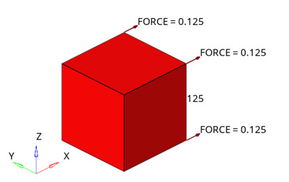
Figure 2. CHEXA element model with applied tensile forces


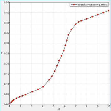
Figure 3. Experimental uniaxial tensile stress-stretch curve

Tensile input data covers engineering stress up to 0.46 MPa and since the design load corresponds to nominal stress of 0.5 MPa, extrapolation is used at the end of the NLSTAT LGDISP load step.

Marlow’s model uses scalar functions instead of scalar parameters to define the material behavior. The model assumes that the strain energy density is independent of the second deviatoric strain invariant and can be decomposed into a deviatoric and a volumetric part. The volumetric part becomes relevant in confined compression.(1) U( I1, I2, J ) = Udev(  I1 ) + Uvol( J ) MathType@MTEF@5@5@+= feaagKart1ev2aaatCvAUfeBSjuyZL2yd9gzLbvyNv2CaerbuLwBLn hiov2DGi1BTfMBaeXatLxBI9gBaerbd9wDYLwzYbItLDharqqtubsr 4rNCHbGeaGqipu0Je9sqqrpepC0xbbL8F4rqqrFfpeea0xe9Lq=Jc9 vqaqpepm0xbba9pwe9Q8fs0=yqaqpepae9pg0FirpepeKkFr0xfr=x fr=xb9adbaqaaeGaciGaaiaabeqaamaabaabaaGcbaaeaaaaaaaaa8 qacaWGvbWdamaabmaabaWdbiaadMeacaaIXaGaaiilaiaabccacaWG jbGaaGOmaiaacYcacaqGGaGaamOsaaWdaiaawIcacaGLPaaapeGaae iiaiabg2da9iaabccacaWGvbGaamizaiaadwgacaWG2bWdamaabmaa baWdbiaabccacaWGjbGaaGymaaWdaiaawIcacaGLPaaapeGaaeiiai abgUcaRiaabccacaWGvbGaamODaiaad+gacaWGSbWdamaabmaabaWd biaadQeaa8aacaGLOaGaayzkaaaaaa@516E@
In case of incompressible deformation, the elastic potential is essentially defined by a single scalar function U d e v MathType@MTEF@5@5@+= feaagKart1ev2aaatCvAUfeBSjuyZL2yd9gzLbvyNv2CaerbuLwBLn hiov2DGi1BTfMBaeXatLxBI9gBaerbd9wDYLwzYbItLDharqqtubsr 4rNCHbGeaGqipu0Je9sqqrpepC0xbbL8F4rqqrFfpeea0xe9Lq=Jc9 vqaqpepm0xbba9pwe9Q8fs0=yqaqpepae9pg0FirpepeKkFr0xfr=x fr=xb9adbaqaaeGaciGaaiaabeqaamaabaabaaGcbaaeaaaaaaaaa8 qacaWGvbGaamizaiaadwgacaWG2baaaa@399E@ . This function is uniquely determined by the stress–strain response measured in a single test, for example, a uniaxial tensile test. MATHEs can be compressible or nearly incompressible, specify nu or D1 to have constant volumetric response throughout the deformation.


Figure 4. Poisson’s ratio, and density of material and reference to the table

Results

The peak deformation in uniaxial tensile test of hyperelastic material with CHEXA element is 13.09 mm.


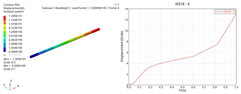
Figure 5. Deformation of CHEXA element due to tensile forces

MATHE Compression


Figure 6. CHEXA element model with compressive forces

The nominal compressive stress of 0.05 MPa is applied with forces. The model is simply supported.

The volumetric part U v o l MathType@MTEF@5@5@+= feaagKart1ev2aaatCvAUfeBSjuyZL2yd9gzLbvyNv2CaerbuLwBLn hiov2DGi1BTfMBaeXatLxBI9gBaerbd9wDYLwzYbItLDharqqtubsr 4rNCHbGeaGqipu0Je9sqqrpepC0xbbL8F4rqqrFfpeea0xe9Lq=Jc9 vqaqpepm0xbba9pwe9Q8fs0=yqaqpepae9pg0FirpepeKkFr0xfr=x fr=xb9adbaqaaeGaciGaaiaabeqaamaabaabaaGcbaaeaaaaaaaaa8 qacaWGvbGaamizaiaadwgacaWG2baaaa@399E@ is considered. Since free lateral expansion is allowed, it has less significance. The volumetric part of the potential of a compressible model can be derived from a stress–strain curve of hydrostatic compression tests. This is defined in TABD where volumetric ratio is specified as a function of pressure. Once U v o l MathType@MTEF@5@5@+= feaagKart1ev2aaatCvAUfeBSjuyZL2yd9gzLbvyNv2CaerbuLwBLn hiov2DGi1BTfMBaeXatLxBI9gBaerbd9wDYLwzYbItLDharqqtubsr 4rNCHbGeaGqipu0Je9sqqrpepC0xbbL8F4rqqrFfpeea0xe9Lq=Jc9 vqaqpepm0xbba9pwe9Q8fs0=yqaqpepae9pg0FirpepeKkFr0xfr=x fr=xb9adbaqaaeGaciGaaiaabeqaamaabaabaaGcbaaeaaaaaaaaa8 qacaWGvbGaamizaiaadwgacaWG2baaaa@399E@ has been determined, U d e v MathType@MTEF@5@5@+= feaagKart1ev2aaatCvAUfeBSjuyZL2yd9gzLbvyNv2CaerbuLwBLn hiov2DGi1BTfMBaeXatLxBI9gBaerbd9wDYLwzYbItLDharqqtubsr 4rNCHbGeaGqipu0Je9sqqrpepC0xbbL8F4rqqrFfpeea0xe9Lq=Jc9 vqaqpepm0xbba9pwe9Q8fs0=yqaqpepae9pg0FirpepeKkFr0xfr=x fr=xb9adbaqaaeGaciGaaiaabeqaamaabaabaaGcbaaeaaaaaaaaa8 qacaWGvbGaamizaiaadwgacaWG2baaaa@399E@ can be obtained from standard compression test considering the volumetric behavior. This approach enables a user-friendly implementation of the Marlow model. You will define the deviatoric and volumetric behavior in tabular form: the test data of a uniaxial, biaxial, or planar test; and for compressible models, additionally, the test data of a volumetric test. In these examples TABD is not used; instead, Poisson’s ratio is specified. Deformation level independent volumetric behavior is internally derived from the initial shear stiffness (TAB1) and Poisson’s ratio.


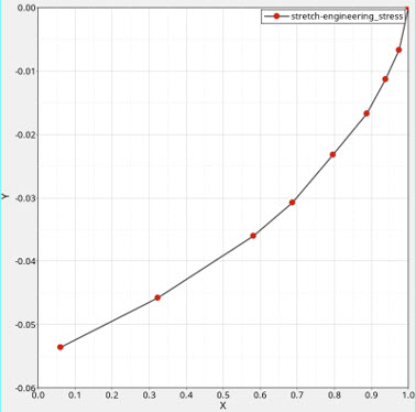
Figure 7. Experimental compressive stress-stretch curve

In compression, stretch can be defined as 0 < λ 1 MathType@MTEF@5@5@+= feaagKart1ev2aaatCvAUfeBSjuyZL2yd9gzLbvyNv2CaerbuLwBLn hiov2DGi1BTfMBaeXatLxBI9gBaerbd9wDYLwzYbItLDharqqtubsr 4rNCHbGeaGqipu0Je9sqqrpepC0xbbL8F4rqqrFfpeea0xe9Lq=Jc9 vqaqpepm0xbba9pwe9Q8fs0=yqaqpepae9pg0FirpepeKkFr0xfr=x fr=xb9adbaqaaeGaciGaaiaabeqaamaabaabaaGcbaGaaGimaiabgY da8iabeU7aSjabgsMiJkaaigdaaaa@3BB8@ and the deformation of the model stays in the specified range.

Results

Hyperelastic Marlow model of CHEXA element shows peak displacement of 0.8185 mm in x-direction.


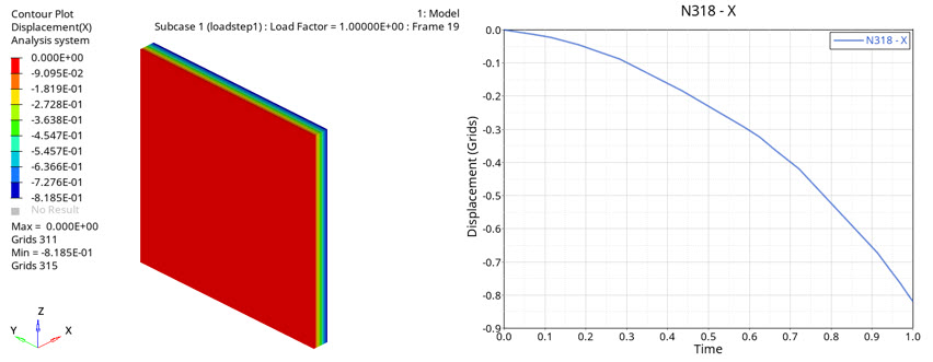
Figure 8. Deformation of CHEXA element due to compression forces

MATTHE

MATTHE is used to define temperature dependent hyperelastic materials. MATTHE is supported in implicit LGDISP analysis. Experimental engineering stress-stretch data at each temperature is presented in tabular format in ascending order.


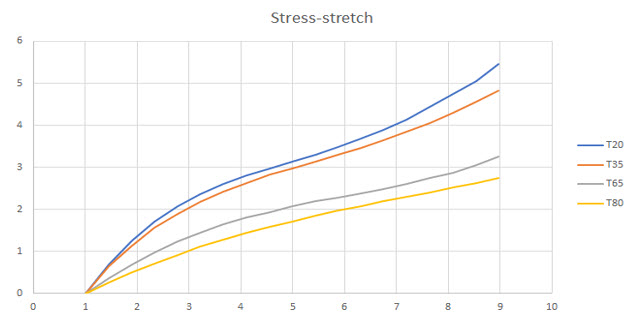
Figure 9. Experimental stress-stretch curve at each temperature


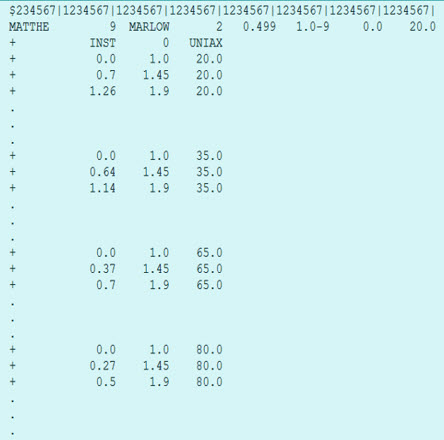
Figure 10. Specify the MATTHE Marlow material model
While defining Marlow material model in OptiStruct, when volumetric behavior is temperature independent, the 1st column corresponds to nominal stress, 2nd to stretch and 3rd to temperature. In this case, either nu (or D1) defines the constant volumetric response throughout the deformation.


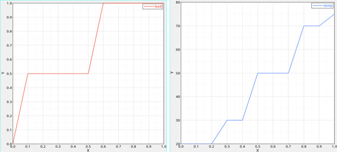
Figure 11. Mechanical load (left) and Thermal load (right) applied on CHEXA element

The example model contains two TLOAD1s that define mechanical and thermal load profiles that evolve in different phases and those are combined with DLOAD.

Results

Hyperelastic MATTHE Marlow model of CHEXA element shows peak displacement of 4.636 mm in x-direction.


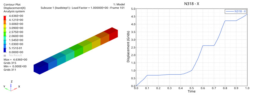
Figure 12. Deformation of CHEXA element. displacement in loading direction

MATHE+VE

A combination of the hyperelastic Marlow model with viscoelasticity provides the capability to describe the strain-rate-dependent material behavior while preserving the advantages of Marlow’s approach, the convenient definition using test data directly and the exact modeling of the test data. Viscoelastic models allow to describe relaxation and strain-rate-dependent elastic properties.

Considering a shear deformation, an integral formulation of linear small strain viscoelasticity is given by:(2) τ( t )= 0 t G( ts ) dγ( s ) dt ds MathType@MTEF@5@5@+= feaagKart1ev2aaatCvAUfeBSjuyZL2yd9gzLbvyNv2CaerbuLwBLn hiov2DGi1BTfMBaeXatLxBI9gBaerbd9wDYLwzYbItLDharqqtubsr 4rNCHbGeaGqiVu0Je9sqqrpepC0xbbL8F4rqqrFfpeea0xe9Lq=Jc9 vqaqpepm0xbba9pwe9Q8fs0=yqaqpepae9pg0FirpepeKkFr0xfr=x fr=xb9adbaqaaeGaciGaaiaabeqaamaabaabaaGcbaGaeqiXdq3aae WaaeaacaWG0baacaGLOaGaayzkaaGaeyypa0Zaa8qCaeaacaWGhbWa aeWaaeaacaWG0bGaeyOeI0Iaam4CaaGaayjkaiaawMcaamaalaaaba Gaamizaiabeo7aNnaabmaabaGaam4CaaGaayjkaiaawMcaaaqaaiaa dsgacaWG0baaaaWcbaGaaGimaaqaaiaadshaa0Gaey4kIipakiaads gacaWGZbaaaa@4D80@
Where,
τ
Shear stress
γ
Shear strain
G ( t ) MathType@MTEF@5@5@+= feaagKart1ev2aaatCvAUfeBSjuyZL2yd9gzLbvyNv2CaerbuLwBLn hiov2DGi1BTfMBaeXatLxBI9gBaerbd9wDYLwzYbItLDharqqtubsr 4rNCHbGeaGqipu0Je9sqqrpepC0xbbL8F4rqqrFfpeea0xe9Lq=Jc9 vqaqpepm0xbba9pwe9Q8fs0=yqaqpepae9pg0FirpepeKkFr0xfr=x fr=xb9adbaqaaeGaciGaaiaabeqaamaabaabaaGcbaGaam4zamaabm aabaGaamiDaaGaayjkaiaawMcaaaaa@3944@
Relaxation function
This can be expressed using the instantaneous shear modulus G 0 MathType@MTEF@5@5@+= feaagKart1ev2aaatCvAUfeBSjuyZL2yd9gzLbvyNv2CaerbuLwBLn hiov2DGi1BTfMBaeXatLxBI9gBaerbd9wDYLwzYbItLDharqqtubsr 4rNCHbGeaGqipu0Je9sqqrpepC0xbbL8F4rqqrFfpeea0xe9Lq=Jc9 vqaqpepm0xbba9pwe9Q8fs0=yqaqpepae9pg0FirpepeKkFr0xfr=x fr=xb9adbaqaaeGaciGaaiaabeqaamaabaabaaGcbaGaam4ramaaBa aaleaacaaIWaaabeaaaaa@3788@ and a relative relaxation function g ( t ) MathType@MTEF@5@5@+= feaagKart1ev2aaatCvAUfeBSjuyZL2yd9gzLbvyNv2CaerbuLwBLn hiov2DGi1BTfMBaeXatLxBI9gBaerbd9wDYLwzYbItLDharqqtubsr 4rNCHbGeaGqipu0Je9sqqrpepC0xbbL8F4rqqrFfpeea0xe9Lq=Jc9 vqaqpepm0xbba9pwe9Q8fs0=yqaqpepae9pg0FirpepeKkFr0xfr=x fr=xb9adbaqaaeGaciGaaiaabeqaamaabaabaaGcbaGaam4zamaabm aabaGaamiDaaGaayjkaiaawMcaaaaa@3944@ by:(3) τ ( t ) = G 0 t g ( t s ) d γ ( s ) d t d s MathType@MTEF@5@5@+= feaagKart1ev2aaatCvAUfeBSjuyZL2yd9gzLbvyNv2CaerbuLwBLn hiov2DGi1BTfMBaeXatLxBI9gBaerbd9wDYLwzYbItLDharqqtubsr 4rNCHbGeaGqiVu0Je9sqqrpepC0xbbL8F4rqqrFfpeea0xe9Lq=Jc9 vqaqpepm0xbba9pwe9Q8fs0=yqaqpepae9pg0FirpepeKkFr0xfr=x fr=xb9adbaqaaeGaciGaaiaabeqaamaabaabaaGcbaGaeqiXdq3aae WaaeaacaWG0baacaGLOaGaayzkaaGaeyypa0Jaam4ramaapehabaGa am4zamaabmaabaGaamiDaiabgkHiTiaadohaaiaawIcacaGLPaaada WcaaqaaiaadsgacqaHZoWzdaqadaqaaiaadohaaiaawIcacaGLPaaa aeaacaWGKbGaamiDaaaaaSqaaiaaicdaaeaacaWG0baaniabgUIiYd GccaWGKbGaam4Caaaa@4E6C@
Usually, the relaxation function is expressed by a Prony series containing N MathType@MTEF@5@5@+= feaagKart1ev2aaatCvAUfeBSjuyZL2yd9gzLbvyNv2CaerbuLwBLn hiov2DGi1BTfMBaeXatLxBI9gBaerbd9wDYLwzYbItLDharqqtubsr 4rNCHbGeaGqipu0Je9sqqrpepC0xbbL8F4rqqrFfpeea0xe9Lq=Jc9 vqaqpepm0xbba9pwe9Q8fs0=yqaqpepae9pg0FirpepeKkFr0xfr=x fr=xb9adbaqaaeGaciGaaiaabeqaamaabaabaaGcbaGaamOtaaaa@36A9@ relaxation times τ i and coefficients g i MathType@MTEF@5@5@+= feaagKart1ev2aaatCvAUfeBSjuyZL2yd9gzLbvyNv2CaerbuLwBLn hiov2DGi1BTfMBaeXatLxBI9gBaerbd9wDYLwzYbItLDharqqtubsr 4rNCHbGeaGqipu0Je9sqqrpepC0xbbL8F4rqqrFfpeea0xe9Lq=Jc9 vqaqpepm0xbba9pwe9Q8fs0=yqaqpepae9pg0FirpepeKkFr0xfr=x fr=xb9adbaqaaeGaciGaaiaabeqaamaabaabaaGcbaGaam4zamaaBa aaleaacaWGPbaabeaaaaa@37DC@ as parameters.(4) g ( t ) = 1 i = 1 N g i ( 1 e t τ i ) MathType@MTEF@5@5@+= feaagKart1ev2aaatCvAUfeBSjuyZL2yd9gzLbvyNv2CaerbuLwBLn hiov2DGi1BTfMBaeXatLxBI9gBaerbd9wDYLwzYbItLDharqqtubsr 4rNCHbGeaGqiVu0Je9sqqrpepC0xbbL8F4rqqrFfpeea0xe9Lq=Jc9 vqaqpepm0xbba9pwe9Q8fs0=yqaqpepae9pg0FirpepeKkFr0xfr=x fr=xb9adbaqaaeGaciGaaiaabeqaamaabaabaaGcbaGaam4zamaabm aabaGaamiDaaGaayjkaiaawMcaaiabg2da9iaaigdacqGHsisldaae WbqaaiaadEgadaWgaaWcbaGaamyAaaqabaGcdaqadaqaaiaaigdacq GHsislcaWGLbWaaWbaaSqabeaacqGHsisldaWcaaqaaiaadshaaeaa cqaHepaDdaWgaaadbaGaamyAaaqabaaaaaaaaOGaayjkaiaawMcaaa WcbaGaamyAaiabg2da9iaaigdaaeaacaWGobaaniabggHiLdaaaa@4D0E@
The Prony series parameters can be obtained from a relaxation test, where a constant strain is applied instantly and the relaxation of the stress over time is measured. A straightforward evaluation of this test is to interpret the normalized stress over time as the normalized relaxation function and to fit it using the Prony series. This approach assumes that the decrease of the normalized stress over time is not significantly influenced by the nonlinearity of the hyperelastic part of the material model.
Table 1. Prony series parameters and bulk modulus of the example
g 1 MathType@MTEF@5@5@+= feaagKart1ev2aaatCvAUfeBSjuyZL2yd9gzLbvyNv2CaerbuLwBLn hiov2DGi1BTfMBaeXatLxBI9gBaerbd9wDYLwzYbItLDharqqtubsr 4rNCHbGeaGqipu0Je9sqqrpepC0xbbL8F4rqqrFfpeea0xe9Lq=Jc9 vqaqpepm0xbba9pwe9Q8fs0=yqaqpepae9pg0FirpepeKkFr0xfr=x fr=xb9adbaqaaeGaciGaaiaabeqaamaabaabaaGcbaGaam4zamaaBa aaleaacaaIXaaabeaaaaa@37A9@ τ 1 MathType@MTEF@5@5@+= feaagKart1ev2aaatCvAUfeBSjuyZL2yd9gzLbvyNv2CaerbuLwBLn hiov2DGi1BTfMBaeXatLxBI9gBaerbd9wDYLwzYbItLDharqqtubsr 4rNCHbGeaGqipu0Je9sqqrpepC0xbbL8F4rqqrFfpeea0xe9Lq=Jc9 vqaqpepm0xbba9pwe9Q8fs0=yqaqpepae9pg0FirpepeKkFr0xfr=x fr=xb9adbaqaaeGaciGaaiaabeqaamaabaabaaGcbaGaeqiXdq3aaS baaSqaaiaaigdaaeqaaaaa@3882@ in s g 2 MathType@MTEF@5@5@+= feaagKart1ev2aaatCvAUfeBSjuyZL2yd9gzLbvyNv2CaerbuLwBLn hiov2DGi1BTfMBaeXatLxBI9gBaerbd9wDYLwzYbItLDharqqtubsr 4rNCHbGeaGqipu0Je9sqqrpepC0xbbL8F4rqqrFfpeea0xe9Lq=Jc9 vqaqpepm0xbba9pwe9Q8fs0=yqaqpepae9pg0FirpepeKkFr0xfr=x fr=xb9adbaqaaeGaciGaaiaabeqaamaabaabaaGcbaGaam4zamaaBa aaleaacaaIXaaabeaaaaa@37A9@ τ 2 MathType@MTEF@5@5@+= feaagKart1ev2aaatCvAUfeBSjuyZL2yd9gzLbvyNv2CaerbuLwBLn hiov2DGi1BTfMBaeXatLxBI9gBaerbd9wDYLwzYbItLDharqqtubsr 4rNCHbGeaGqipu0Je9sqqrpepC0xbbL8F4rqqrFfpeea0xe9Lq=Jc9 vqaqpepm0xbba9pwe9Q8fs0=yqaqpepae9pg0FirpepeKkFr0xfr=x fr=xb9adbaqaaeGaciGaaiaabeqaamaabaabaaGcbaGaeqiXdq3aaS baaSqaaiaaigdaaeqaaaaa@3882@ in s g 3 MathType@MTEF@5@5@+= feaagKart1ev2aaatCvAUfeBSjuyZL2yd9gzLbvyNv2CaerbuLwBLn hiov2DGi1BTfMBaeXatLxBI9gBaerbd9wDYLwzYbItLDharqqtubsr 4rNCHbGeaGqipu0Je9sqqrpepC0xbbL8F4rqqrFfpeea0xe9Lq=Jc9 vqaqpepm0xbba9pwe9Q8fs0=yqaqpepae9pg0FirpepeKkFr0xfr=x fr=xb9adbaqaaeGaciGaaiaabeqaamaabaabaaGcbaGaam4zamaaBa aaleaacaaIXaaabeaaaaa@37A9@ τ 3 MathType@MTEF@5@5@+= feaagKart1ev2aaatCvAUfeBSjuyZL2yd9gzLbvyNv2CaerbuLwBLn hiov2DGi1BTfMBaeXatLxBI9gBaerbd9wDYLwzYbItLDharqqtubsr 4rNCHbGeaGqipu0Je9sqqrpepC0xbbL8F4rqqrFfpeea0xe9Lq=Jc9 vqaqpepm0xbba9pwe9Q8fs0=yqaqpepae9pg0FirpepeKkFr0xfr=x fr=xb9adbaqaaeGaciGaaiaabeqaamaabaabaaGcbaGaeqiXdq3aaS baaSqaaiaaigdaaeqaaaaa@3882@ in s g 4 MathType@MTEF@5@5@+= feaagKart1ev2aaatCvAUfeBSjuyZL2yd9gzLbvyNv2CaerbuLwBLn hiov2DGi1BTfMBaeXatLxBI9gBaerbd9wDYLwzYbItLDharqqtubsr 4rNCHbGeaGqipu0Je9sqqrpepC0xbbL8F4rqqrFfpeea0xe9Lq=Jc9 vqaqpepm0xbba9pwe9Q8fs0=yqaqpepae9pg0FirpepeKkFr0xfr=x fr=xb9adbaqaaeGaciGaaiaabeqaamaabaabaaGcbaGaam4zamaaBa aaleaacaaIXaaabeaaaaa@37A9@ τ 4 MathType@MTEF@5@5@+= feaagKart1ev2aaatCvAUfeBSjuyZL2yd9gzLbvyNv2CaerbuLwBLn hiov2DGi1BTfMBaeXatLxBI9gBaerbd9wDYLwzYbItLDharqqtubsr 4rNCHbGeaGqipu0Je9sqqrpepC0xbbL8F4rqqrFfpeea0xe9Lq=Jc9 vqaqpepm0xbba9pwe9Q8fs0=yqaqpepae9pg0FirpepeKkFr0xfr=x fr=xb9adbaqaaeGaciGaaiaabeqaamaabaabaaGcbaGaeqiXdq3aaS baaSqaaiaaigdaaeqaaaaa@3882@ in s g 5 MathType@MTEF@5@5@+= feaagKart1ev2aaatCvAUfeBSjuyZL2yd9gzLbvyNv2CaerbuLwBLn hiov2DGi1BTfMBaeXatLxBI9gBaerbd9wDYLwzYbItLDharqqtubsr 4rNCHbGeaGqipu0Je9sqqrpepC0xbbL8F4rqqrFfpeea0xe9Lq=Jc9 vqaqpepm0xbba9pwe9Q8fs0=yqaqpepae9pg0FirpepeKkFr0xfr=x fr=xb9adbaqaaeGaciGaaiaabeqaamaabaabaaGcbaGaam4zamaaBa aaleaacaaIXaaabeaaaaa@37A9@ τ 5 MathType@MTEF@5@5@+= feaagKart1ev2aaatCvAUfeBSjuyZL2yd9gzLbvyNv2CaerbuLwBLn hiov2DGi1BTfMBaeXatLxBI9gBaerbd9wDYLwzYbItLDharqqtubsr 4rNCHbGeaGqipu0Je9sqqrpepC0xbbL8F4rqqrFfpeea0xe9Lq=Jc9 vqaqpepm0xbba9pwe9Q8fs0=yqaqpepae9pg0FirpepeKkFr0xfr=x fr=xb9adbaqaaeGaciGaaiaabeqaamaabaabaaGcbaGaeqiXdq3aaS baaSqaaiaaigdaaeqaaaaa@3882@ in s K of GPa
0.3539 0.08124 0.07458 1.692 0.05052 35.23 0.04117 733.5 0.04575 15275 2.5
When viscoelasticity is considered, moduli temporal property needs to be specified in the continuation line of MATHE card. By default, this is considered as long-term relaxed input. The other options are to specify it as instantaneous input. MATVE card has the same ID as MATHE.


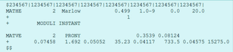
Figure 13. MATHE + MATVE card specification with same ID for visco-hyperelastic model
According to the definition of the visco-hyperelastic model, it requires to specify the parameters of the Prony series as well as to specify the temporal (here instantaneous) hyperelastic response by the potential U0. It is the response that the model shows on a timescale much smaller than the lowest considered relaxation time. This timescale lies outside the validity range of the model, so U0 does not have the physical meaning of the high frequency limit of the real material behavior. Nevertheless, U0 must be identified from experimental data to specify the model. It is basically a transformation from a uniaxial stress–strain curve at constant strain rate to the curve describing the instantaneous hyperelastic response.


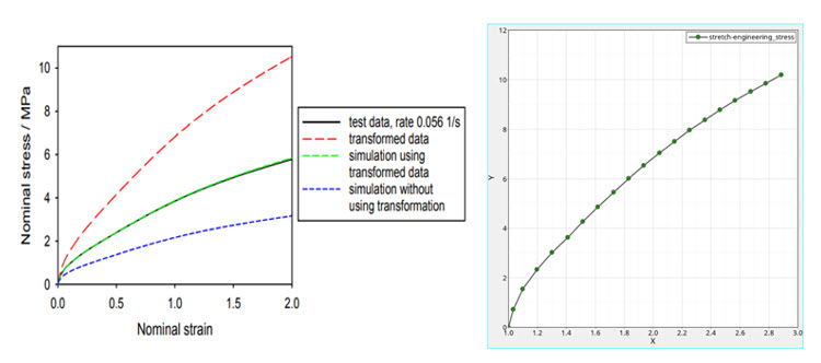
Figure 14. Instantaneous stress-strain curve (left) and the corresponding stress-stretch curve for the MATHE card (right)
The red dashed curve is the instantaneous stress–strain curve of the viscoelastic Marlow model. The example model takes the stress-stretch data as instantaneous definition for MATHE and uses Prony series to define viscoelastic behavior.


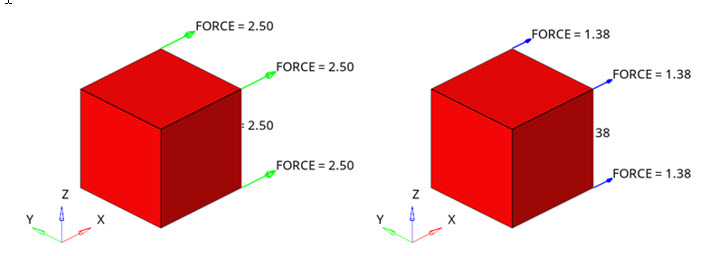
Figure 15. Two loadsteps with different loads and loading rates

Single element model is uniaxially loaded from zero to nominal stress. First loadstep having 10.0 MPa of nominal stress ramped within 0.02s (left) and second loadstep with 5.5 MPa of nominal stress ramped within 200s (right).

Results

Both load steps return the same displacement of 2 mm at the end of the nonlinear transient analysis. Nominal strain matches with reference result.


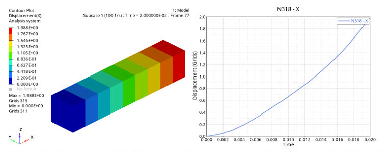
Figure 16. Deformation of CHEXA element from unloaded state to nominal 10.0 MPa within 0.02s


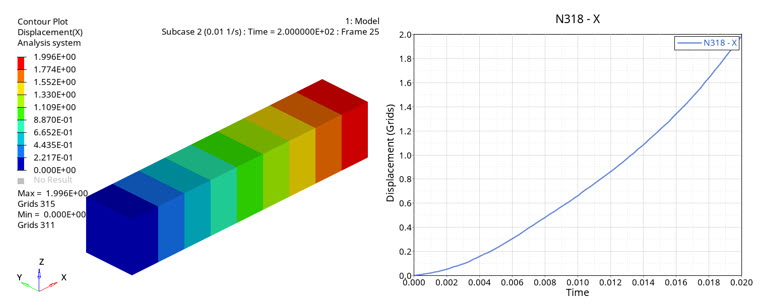
Figure 17. Deformation of CHEXA element from unloaded state to nominal 5.5 MPa within 200s


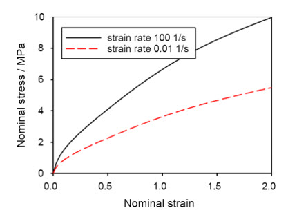
Figure 18. Reference results

MATTHE+VE

The model contains three cubes represented with CTETRA, CPENTA and CHEXA elements. Models are loaded with different strain rates up to 30% deformation level and then hold so that the total analysis time in nonlinear transient is 147s. Analysis environment is T=100°C and input data is given at T=80°C and T=120°C, respectively.


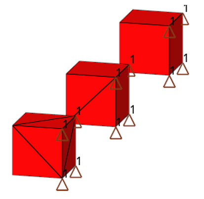
Figure 19. CTETRA, CPENTA and CHEXA model elements
Temperature dependent Marlow model with viscoelasticity combines previously described material definitions. Temperature dependent MATTHE is defined in tabular format. Rate-dependency described in MATVE is common for all environments.


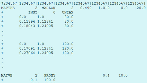
Figure 20. Temperature dependent MATTHE Marlow model
The example models take the widely referred Treloar’s stress-stretch data as reference and this is considered to return the baseline solution at T=100°C. Stress values are multiplied by factors 0.8 and 1.2 to obtain stress-stretch data at two extrapolated environments.


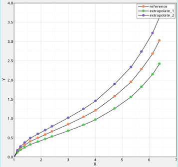
Figure 21. Stress-stretch data of the material


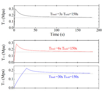
Figure 22. Reference result with 3s, 6s and 30s Tload

The uniaxial tension data at the two extrapolated environments is used as the input data.

Results

MATTHE with MARLOW + VE returns a good match for stress relaxation against the published results. In the reference study OGDEN MATHE was used (single environment). OptiStruct MATHE(OGDEN) +VE perfectly matches the simulation results shown in the reference.


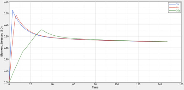
Figure 23. Elemental stresses with 3s, 6s, and 30s Tload
1 Transformation of Test Data for the Specification of a Viscoelastic Marlow Model. Olaf Hesebeck, Fraunhofer Institute for Manufacturing Technology and Advanced Materials IFAM, Wiener Straße 12, 28359 Bremen, Germany.
2 Parameter Identification Methods for Hyperelastic and Hyper-Viscoelastic Models. Yifeng Wu, Hao Wang, and Aiqun Li. School of Civil Engineering, Southeast University, Nanjing 210096, China, Beijing University of Civil Engineering and Architecture, Beijing 100044, China