Materials

The different material types provided by OptiStruct are: isotropic, orthotropic, and anisotropic materials. The material property definition cards are used to define the properties for each of the materials used in a structural model.

The MAT1 Bulk Data Entry is used to define the properties for isotropic elastic materials. It can be referenced by any of the structural elements and can also be referenced by any property card.

The MAT2 entry is used to define the properties for anisotropic materials. It applies only to triangular or quadrilateral membrane and bending elements, and can only be referenced by PSHELL, PCOMP, and PCOMPG property cards. This material type specifies the relationship between the in-plane stresses and strains. The angle between the material coordinate system and the element coordinate system is specified on the connection cards.

The MAT3 entry is used to define the material properties for axisymmetric and plane-strain elements. It can be referenced by CTRIAX6 elements and can also be referenced by any PAXI property card which is in turn referenced on CTAXI or CQAXI elements. Similarly, it can be referenced by the PPLANE property which is referenced by plane-strain CQPSTN and CTPSTN elements.

The MAT4 entry is used to define the isotropic thermal material properties. It can be referenced by any of the structural elements, and can also be referenced by any property card.

The MAT5 entry is used to define the anisotropic thermal material properties. It can be referenced by any of the structural elements and can also be referenced by any property card.

The MAT8 card is used to define the properties for planar orthotropic elastic materials in two dimensions. Individual plys of a layered composite lay-up typically possess such orthotropic properties. Since layered composite laminates are modeled using shell elements, MAT8 property data can only be referenced by PSHELL, PCOMP, and PCOMPG property cards.

The MAT9 Bulk Data Entry can be used to define the properties for anisotropic elastic materials for three dimensional solid elements. The general an-isotropic stress-strain relationship linking the six independent stress components of the stress tensor at a point and the six independent strain components of the tensor at the point contain 21 independent constants in the elasticity matrix. These values are supplied using the MAT9 Bulk Data card. The MAT9 Bulk Data card is used with the CHEXA, CPENTA, CPYRA, and CTETRA solid elements, and can only be referenced on the PSOLID property card. The optional coordinate system in which MAT9 data are specified is supplied via the PSOLID Bulk Data Entry.

The MAT10 Bulk Data Entry is used to define material properties for fluid elements in coupled fluid-structural (acoustic) analysis. It may only be referenced on PSOLID entries with FCTN=PFLUID.

Biot (poroelastic) material is defined using MATPE1 entry.

Temperature dependent material properties are defined using MATT1, MATT2, MATT8, and MATT9. All four have the same characteristics as described above. The temperature dependency of each property is defined through TABLEM1, TABLEM2, TABLEM3, or TABLEM4 table entries.

Composite Laminates are defined using the PCOMP, PCOMPP and PCOMPG properties. They are not material types; each ply in the laminate lay-up can reference a different material.

Elasto-plastic material properties are defined using MATS1. The nonlinear material characteristics may need the table input TABLES1. MATS1 is defined as an extension to a MAT1 with the same MID. MATS1 is applicable to all nonlinear solutions.

Hyperelastic material properties are defined using MATHE. Various Hyperelastic material models are available, such are Ogden, Arruda-Boyce, and so on.

Viscoelastic material properties are defined using MATVE or MATFVE, if frequency-dependency is required.

Creep material properties are defined using MATVP.

Cohesive Zone Modeling can be defined using MCOHE or MCOHED entries.

Cast Iron Plasticity material can be defined using MCIRON Bulk Data Entry.

User-defined structural material properties are available using MATUSR. .dll or .so libraries can be referenced via the LOADLIB entry. For more information, refer to User-Defined Structural Material in the User Guide.

User-defined thermal material properties are available using MATUSHT. .dll or .so libraries can be referenced via the LOADLIB entry.

Material models can also be defined using Multiscale Designer and used via the MATMDS entry.

For explicit dynamic subcases (with Radioss integration), more nonlinear material laws are available. As a general rule, material definitions that are only applicable in explicit dynamic analysis are defined on extensions to a MAT1 material that defines the basic elastic properties. The extensions are grouped with the base entry by sharing the same MID. The MATXyx extensions available are listed below. If a law requires material curves, TABLES1 entries are used.
Table 1. Implicit Analysis
Material Property Nonlinearity Time-dependency Temperature-dependency Frequency-dependency Material Card
Isotropic - - - - MAT1
- - - Yes MAT1 + MATF1
- - Yes - MAT1 + MATT1
Elasto-plasticity - - - MAT1 + MATS1
- Yes - MAT1 + MATS1 (referencing TABLEST)
Hyperelasticity - - - MATHE
- Yes - MATTHE
Viscoelasticity - - - MAT1 + MATVE
- - Yes MAT1 + MATFVE
Viscoelasticity, Hyperelasticity - - - MATHE + MATVE
Creep - - - MAT1 + MATVP
Creep, Elasto-plasticity - - - MAT1 + MATVP + MATS1
Creep - Yes - MAT1 + MATVP + MATTVP
Anisotropic - - - - MAT9 (solid elements)

MAT2 (shell elements)

- - - Yes MAT9 + MATF9 (solid elements)

MAT2 + MATF2 (shell elements)

- - Yes - MAT9 + MATT9 (solid elements)

MAT2 + MATT2 (shell elements)

Viscoelasticity - - - MAT9 + MATVE
- - Yes MAT9 + MATFVE
Orthotropic - - - - MAT9OR (solid elements)

MAT8 (shell elements)

MAT3 (axisymmetric and plane strain elements)

- - - Yes MAT8 + MATF8 (shell elements)

MAT3 + MATF3 (axisymmetric and plane strain elements)

- - Yes - MAT9OR + MATT9OR (solid elements)

MAT8 + MATT8 (shell elements)

MAT3 + MATT3 (axisymmetric and plane strain elements)

Fluid - - - - MAT10
- - - Yes MAT10 + MATF10
Thermal - - - - MAT4 (Isotropic)

MAT5 (Anisotropic)

Yes (Temperature) - Yes - MAT4 + MATT4 (Isotropic)
Gasket - - Yes - MGASK
Fatigue - - - - MATFAT
Biot (Poroelasticity) - - - - MATPE1
User-Defined Structural Material Subroutines Yes Yes Yes - MATUSR (Fortran and C for subroutines)
User-Defined Thermal Material Subroutines Yes (Temperature) Yes Yes - MATUSHT (Fortran and C for subroutines)
Multiscale Designer-based Material Yes - - - MATMDS (using Altair Multiscale Designer).
Failure Criteria - - - - Criteria and Allowables on MATF

Criteria/Allowables can also be defined on MAT1, MAT2, MAT8, PCOMP, PCOMPP, PCOMPG

Table 2. Explicit Dynamic Analysis
Material Property Nonlinearity Time-dependency Temperature-dependency Frequency-dependency Material Card
Isotropic - - - - MAT1
Elasto-plasticity - - - MAT1 + MATS1
Hyperelasticity - - - MATHE
Viscoelasticity - - - MAT1 + MATVE
Viscoelasticity, Hyperelasticity - - - MATHE + MATVE
Anisotropic - - - - MAT2 (shell elements)
Viscoelasticity - - - MAT9 + MATVE
Orthotropic - - - - MAT8 (shell elements)

For explicit dynamic subcases (with Radioss integration), more nonlinear material laws are available. As a general rule, material definitions that are only applicable in explicit dynamic analysis are defined on extensions to a MAT1 material that defines the basic elastic properties. The extensions are grouped with the base entry by sharing the same MID. The MATXyz extensions available are listed below. If a law requires material curves, TABLES1 entries are used.

Explicit Dynamic Analysis (Radioss Integration via ANALYSIS=EXPDYN)

Material Card
Description
MATX0
Void material
MATX02
Johnson-Cook elastic-plastic material
MATX13
Rigid material
MATX21
Rock-Concrete material
MATX25
Composite shell material, TSAI-WU and CRASURV formulations
MATX27
Brittle elastic-plastic material
MATX28
Honeycomb material
MATX33
Visco-elastic foam material
MATX36
Piece-wise linear elastic-plastic material
MATX42
Ogden-Mooney and Rivlin material
MATX43
Hill orthotropic material
MATX44
Cowper-Symonds elastic-plastic material
MATX60
Piece-wise nonlinear elastic-plastic material
MATX62
Hyper-visco-elastic material
MATX65
Tabulated strain-rate dependent elastic-plastic material
MATX68
Honeycomb material
MATX70
Tabulated visco-elastic foam material
MATX82
Ogden material

User-Defined Structural Material

The MATUSR Bulk Data Entry, in combination with the LOADLIB I/O Option Entry, allows for the definition of structural material through user-defined external functions.

The external functions may be written in Fortran, C or C++. The resulting libraries and files should be accessible by OptiStruct regardless of the coding language, provided that consistent function prototyping is respected, and adequate compiling and linking options are used.

Write External Functions

Two Fortran subroutines are required to define user material in OptiStruct. First, a Nonlinear subroutine for the nonlinear large displacement solution, and another subroutine for the linear and nonlinear small displacement solution. Both subroutines are mandatory, and the same argument order should be followed as:

Nonlinear subroutine (LGDISP):
subroutine usermaterial(idu, stress, strain, dstrain, stater,
state, nstate, drot, props, nprops, ndi, nshear, ntens 
	temp, dtemp, ieuid, kinc, dt, t_step,
	t_total, cdev, cbulk, userdata, ierr)

integer idu, nstate, nprops, kinc, ieuid, ndi, nshear, ntens, ierr
double precision stress(6),stater(*),state(*),
     $     cdev(6,6),cbulk, drot(3,3), temp, dtemp, dt, 
     $     t_step, t_total,
     $     strain(6), dstrain(6), props(nprops)
character*32000 userdata
Linear subroutine (Linear and SMDISP):
subroutine smatusr(idu, nprop, prop, ndi, nshear, ntens, smat, userdata,  ierr)
integer idu, nprop, ndi, nshear, ntens, ierr
double precision prop(nprop), smat(*)
character*32000 userdata
Note: It is important that both subroutines be named “usermaterial” and “smatusr”, respectively.

Subroutine Arguments

The following table briefly describes the arguments which are passed among OptiStruct and the external subroutines. OptiStruct calls these two subroutines for every integration point of every element in the model. Therefore, the values listed below are calculated at each integration point.
Argument Type Input / Output Description
idu integer Input This is defined via the USUBID parameter on the MATUSR Bulk Data Entry. This argument can be used to define and choose between different types of materials within the same user subroutine.

optional use

stress double (table) Input/Output This is the Stress tensor. The initial stress is considered to be input and the stress, tensor calculated during the nonlinear solution are output from the user subroutine to OptiStruct.
strain double (table) Input Strain tensor. The initial strain is considered to be input.
dstrain double (table) Input Incremental strain table. The incremental strain is input from OptiStruct to the user subroutine.
stater double (table) Input/Output Table of State variables at the previous increment.
state double (table) Input/Output Table of State variables at the current increment. See stater for more information. State variables are variables that can be requested as output in the H3D file. Any variable (for example, plastic strain, equivalent plastic strain, and so on) calculated within the solution process in the subroutine can be output by defining it as a state variable. The number of state variables can be specified via nstate.
nstate integer Input/Output Number of State Variables that the user requires in the subroutine. These state variables are output in the H3D file. See stater for more information. This is specified via the NDEPVAR field of the MATUSR Bulk Data Entry.
props double (table) Input This table contains all the user-defined material property information from the PROPERTY continuation line of the MATUSR entry.
nprops Integer Input This is the total number of material properties defined on the PROPERTY continuation line of the MATUSR entry.
ndi Integer Input The number of normal stress components (3 for solid elements, 2 for shell elements).
nshear Integer Input The number of shear stress components (3 for solid elements, 1 for shell elements).
ntens Integer Input The number of tensor components (ntens = ndi + nshear).
temp double Input This is the temperature at the previous converged increment.
dtemp double Input This is the temperature increment.
ieuid integer Input Element ID. This subroutine is called for every integration point for every element.
kinc integer Input Current increment.
dt double Input Current Time increment
t_step double Input Subcase time.
t_total double Input Total time (if CNTNLSUB is used)
cdev double (table) Output Full material modulus matrix of size (6x6). These are calculated during the solution and are output to OptiStruct to form the stiffness matrix.
cbulk double (table) Output (Optional) Bulk material modulus Matrix. This is currently not used in the solution.
smat Double (table) Output 1D array (21 terms). This is the symmetric part of cdev. These are calculated during the solution and are output to OptiStruct to form the stiffness matrix.
userdata Character Output User-defined message that is output based on the value of ierr argument.
ierr Integer Input/Output Flag that activates/deactivates Output message for an OptiStruct run from the user subroutine.
0 (Default)
No action.
1
The OptiStruct run errors out and an ERROR message is printed based on the message defined in userdata argument.
-1
The information message defined in userdata argument is printed and the OptiStruct run continues.

Build External Libraries for User-defined Materials

Allows building shared libraries on Windows or Linux.

Refer to Build External Libraries for more information.

User-Defined Thermal Material

The MATUSHT Bulk Data Entry, in combination with the LOADLIB I/O Option Entry, allows for the definition of thermal material through user-defined external functions.

The external functions may be written in Fortran, C or C++. The resulting libraries and files should be accessible by OptiStruct regardless of the coding language, provided that consistent function prototyping is respected, and adequate compiling and linking options are used.
Note: User-defined Thermal Material Heat Transfer is currently only supported for Nonlinear Transient Heat Transfer Analysis.

Write External Functions

Subroutine:
subroutine usrmatht(idu, matID, ieuid, Stater, State,
 nState, drot, props, nprops, temp, 
 dtemp, kinc, dt, t_step, t_total, hgen, smat
 userdata, ierr)

      character*32000 userdata

integer*8 i, idu, matID, ieuid, nState, nprops, kinc, ierr
      double precision Stater(nState), State(nState)
      double precision drot(3,3), rmat(nprops)
      double precision etempmat, dtemp, dt, t_step, t_total
      double precision hgen, smat(9)

Subroutine Arguments

The following table briefly describes the arguments which are passed among OptiStruct and the external subroutines.
Argument Type Input / Output Description
idu integer Input This is defined via the USUBID parameter on the MATUSHT Bulk Data Entry. This argument can be used to define and choose between different types of materials within the same user subroutine.

optional use

matID Integer Input Material ID.
ieuid integer Input Element ID.
drot(3,3) Double (table) Input Transformation matrix.
props double (table) Input This table contains all the user-defined thermal material property information from the PROPERTY continuation line of the MATUSHT entry.
nprops Integer Input This is the total number of thermal material properties defined on the PROPERTY continuation line of the MATUSHT entry.
temp double Input This is the temperature at the end of the current increment.
dtemp double Input This is the temperature increment of the current increment.
kinc integer Input Current nonlinear increment.
dt double Input Current time step increment
t_step double Input Current subcase time of the current time step.
t_total double Input Total time (if IC is used). This is effective when the IC case control entry of a nonlinear transient thermal subcase points to a previous nonlinear transient thermal subcase.
Stater double (table) Input Table of State variables at the last converged time-step. They are constant between iterations of the same time step.
State double (table) Input/Output Table of State variables at the current time-step. They are updated and passed between iterations of the same time-step. State variables are variables that can be requested as output in the H3D file. Any variable calculated within the solution process in the subroutine can be output by defining it as a state variable.
nState integer Input Number of State Variables that the user requires in the subroutine. See Stater for more information.
hgen double (table) Output Generated heat.
smat Double (table) Output Material matrix. These are calculated during the solution and are output to OptiStruct. Format for smat matrix is provided below.
smat(1): KXX Thermal Conductivity
smat(2): KXY Thermal Conductivity
smat(3): KXZ Thermal Conductivity
smat(4): KYY Thermal Conductivity
smat(5): KYZ Thermal Conductivity
smat(6): KZZ Thermal Conductivity
smat(7): CP Heat Capacity per unit mass
smat(8): RHO Density
smat(9): Free Convection Heat Transfer 
Coefficient (Unused).
userdata Character Output User-defined message that is output based on the value of ierr argument.
ierr Integer Input/Output Flag that activates/deactivates Output message for an OptiStruct run from the user subroutine.
0 (Default)
No action.
1
The OptiStruct run errors out and an ERROR message is printed based on the message defined in userdata argument.
-1
The information message defined in userdata argument is printed and the OptiStruct run continues.

Output

Regular Built-in OptiStruct output, like Grid Temperatures, Element Fluxes, and so on can be requested for any thermal material user-subroutine based model. Additionally, user-defined output can also be requested via the State(*) variable in the user-subroutine. The number of such State(*) variables should be identified on the NDEPVAR field.

This State variable can be assigned to any output variable that is required to be output from the subroutine, and it can then be visualized in HyperView after loading the H3D file.

Build External Libraries for User-defined Materials

You can build shared libraries on Windows or Linux.

Refer to Build External Libraries for more information.

Combined Hardening of von Mises Plasticity

Combining hardening can be used for analysis with cyclic loading, in order to capture shakedown, ratcheting effect, and so on.

It consists of two nonlinear hardening rules, the nonlinear kinematic (NLKIN) and nonlinear isotropic (NLISO) hardening methods.

Generally, the isotropic part is closely related to the von Mises criteria, and the kinematic part is described by the evolution law of back stress.

Combined hardening can be activated by setting HR=6 on the MATS1 Bulk Data.

Isotropic Hardening (NLISO): Nonlinear Yield Function

The yield function of von Mises plasticity can be expressed in a general form as:(1) f(S,α, ε ¯ p )= 3 2 (Sα):(Sα) σ y ( ε ¯ p ) MathType@MTEF@5@5@+= feaagKart1ev2aaatCvAUfeBSjuyZL2yd9gzLbvyNv2CaerbuLwBLn hiov2DGi1BTfMBaeXatLxBI9gBaerbd9wDYLwzYbItLDharqqtubsr 4rNCHbGeaGqiVu0Je9sqqrpepC0xbbL8F4rqqrFfpeea0xe9Lq=Jc9 vqaqpepm0xbba9pwe9Q8fs0=yqaqpepae9pg0FirpepeKkFr0xfr=x fr=xb9adbaqaaeGaciGaaiaabeqaamaabaabaaGcbaGaamOzaiaacI cacaWHtbGaaiilaiaahg7acaGGSaGafqyTduMbaebadaWgaaWcbaGa amiCaaqabaGccaGGPaGaeyypa0ZaaOaaaeaadaWcaaqaaiaaiodaae aacaaIYaaaaiaacIcacaWHtbGaeyOeI0IaaCySdiaacMcacaGG6aGa aiikaiaahofacqGHsislcaWHXoGaaiykaaWcbeaakiabgkHiTiabeo 8aZnaaBaaaleaacaWG5baabeaakiaacIcacuaH1oqzgaqeamaaBaaa leaacaWGWbaabeaakiaacMcaaaa@52F4@
Where,
S MathType@MTEF@5@5@+= feaagKart1ev2aaatCvAUfeBSjuyZL2yd9gzLbvyNv2CaerbuLwBLn hiov2DGi1BTfMBaeXatLxBI9gBaerbd9wDYLwzYbItLDharqqtubsr 4rNCHbGeaGqiVu0Je9sqqrpepC0xbbL8F4rqqrFfpeea0xe9Lq=Jc9 vqaqpepm0xbba9pwe9Q8fs0=yqaqpepae9pg0FirpepeKkFr0xfr=x fr=xb9adbaqaaeGaciGaaiaabeqaamaabaabaaGcbaGaaC4uaaaa@36D2@
Deviatoric stress tensor.
α MathType@MTEF@5@5@+= feaagKart1ev2aaatCvAUfeBSjuyZL2yd9gzLbvyNv2CaerbuLwBLn hiov2DGi1BTfMBaeXatLxBI9gBaerbd9wDYLwzYbItLDharqqtubsr 4rNCHbGeaGqiVu0Je9sqqrpepC0xbbL8F4rqqrFfpeea0xe9Lq=Jc9 vqaqpepm0xbba9pwe9Q8fs0=yqaqpepae9pg0FirpepeKkFr0xfr=x fr=xb9adbaqaaeGaciGaaiaabeqaamaabaabaaGcbaGaaCySdaaa@3733@
Back stress tensor.
σ y MathType@MTEF@5@5@+= feaagKart1ev2aaatCvAUfeBSjuyZL2yd9gzLbvyNv2CaerbuLwBLn hiov2DGi1BTfMBaeXatLxBI9gBaerbd9wDYLwzYbItLDharqqtubsr 4rNCHbGeaGqiVu0Je9sqqrpepC0xbbL8F4rqqrFfpeea0xe9Lq=Jc9 vqaqpepm0xbba9pwe9Q8fs0=yqaqpepae9pg0FirpepeKkFr0xfr=x fr=xb9adbaqaaeGaciGaaiaabeqaamaabaabaaGcbaGaeq4Wdm3aaS baaSqaaiaadMhaaeqaaaaa@38E3@
Yield stress as a function of equivalent plastic strain ε ¯ p MathType@MTEF@5@5@+= feaagKart1ev2aaatCvAUfeBSjuyZL2yd9gzLbvyNv2CaerbuLwBLn hiov2DGi1BTfMBaeXatLxBI9gBaerbd9wDYLwzYbItLDharqqtubsr 4rNCHbGeaGqiVu0Je9sqqrpepC0xbbL8F4rqqrFfpeea0xe9Lq=Jc9 vqaqpepm0xbba9pwe9Q8fs0=yqaqpepae9pg0FirpepeKkFr0xfr=x fr=xb9adbaqaaeGaciGaaiaabeqaamaabaabaaGcbaGafqyTduMbae badaWgaaWcbaGaamiCaaqabaaaaa@38D6@ .
The flow rule is defined as change of plastic strain, expressed in rate form as:(2) ε ˙ p = λ ˙ f σ MathType@MTEF@5@5@+= feaagKart1ev2aaatCvAUfeBSjuyZL2yd9gzLbvyNv2CaerbuLwBLn hiov2DGi1BTfMBaeXatLxBI9gBaerbd9wDYLwzYbItLDharqqtubsr 4rNCHbGeaGqiVu0Je9sqqrpepC0xbbL8F4rqqrFfpeea0xe9Lq=Jc9 vqaqpepm0xbba9pwe9Q8fs0=yqaqpepae9pg0FirpepeKkFr0xfr=x fr=xb9adbaqaaeGaciGaaiaabeqaamaabaabaaGcbaGabCyTdyaaca WaaSbaaSqaaiaadchaaeqaaOGaeyypa0Jafq4UdWMbaiaadaWcaaqa aiabgkGi2kaadAgaaeaacqGHciITcaWHdpaaaaaa@4044@

Where, λ is the rate of plastic multiplier, which is also the rate of equivalent plastic strain.

The flow direction, N MathType@MTEF@5@5@+= feaagKart1ev2aaatCvAUfeBSjuyZL2yd9gzLbvyNv2CaerbuLwBLn hiov2DGi1BTfMBaeXatLxBI9gBaerbd9wDYLwzYbItLDharqqtubsr 4rNCHbGeaGqiVu0Je9sqqrpepC0xbbL8F4rqqrFfpeea0xe9Lq=Jc9 vqaqpepm0xbba9pwe9Q8fs0=yqaqpepae9pg0FirpepeKkFr0xfr=x fr=xb9adbaqaaeGaciGaaiaabeqaamaabaabaaGcbaGaaCOtaaaa@36CD@ can be introduced which is the derivative of the yield function with respect to the stress tensor,(3) N = f σ = 3 2 ( S α ) | | S α | | = 3 2 η | | η | | MathType@MTEF@5@5@+= feaagKart1ev2aaatCvAUfeBSjuyZL2yd9gzLbvyNv2CaerbuLwBLn hiov2DGi1BTfMBaeXatLxBI9gBaerbd9wDYLwzYbItLDharqqtubsr 4rNCHbGeaGqiVu0Je9sqqrpepC0xbbL8F4rqqrFfpeea0xe9Lq=Jc9 vqaqpepm0xbba9pwe9Q8fs0=yqaqpepae9pg0FirpepeKkFr0xfr=x fr=xb9adbaqaaeGaciGaaiaabeqaamaabaabaaGcbaGaaCOtaiabg2 da9maalaaabaGaeyOaIyRaamOzaaqaaiabgkGi2kaaho8aaaGaeyyp a0ZaaOaaaeaadaWcaaqaaiaaiodaaeaacaaIYaaaaaWcbeaakmaala aabaGaaiikaiaahofacqGHsislcaWHXoGaaiykaaqaaiaacYhacaGG 8bGaaC4uaiabgkHiTiaahg7acaGG8bGaaiiFaaaacqGH9aqpdaGcaa qaamaalaaabaGaaG4maaqaaiaaikdaaaaaleqaaOWaaSaaaeaacaWH 3oaabaGaaiiFaiaacYhacaWH3oGaaiiFaiaacYhaaaaaaa@545C@

Where, η is the relative stress tensor, which is the difference between deviatoric stress and back stress.

For the nonlinear isotropic hardening, the yield stress is assumed to be a power law function of equivalent plastic strain:(4) σ y ( ε ¯ p )= σ y0 +Q(1 e b ε ¯ p ) MathType@MTEF@5@5@+= feaagKart1ev2aaatCvAUfeBSjuyZL2yd9gzLbvyNv2CaerbuLwBLn hiov2DGi1BTfMBaeXatLxBI9gBaerbd9wDYLwzYbItLDharqqtubsr 4rNCHbGeaGqiVu0Je9sqqrpepC0xbbL8F4rqqrFfpeea0xe9Lq=Jc9 vqaqpepm0xbba9pwe9Q8fs0=yqaqpepae9pg0FirpepeKkFr0xfr=x fr=xb9adbaqaaeGaciGaaiaabeqaamaabaabaaGcbaGaeq4Wdm3aaS baaSqaaiaadMhaaeqaaOGaaiikaiqbew7aLzaaraWaaSbaaSqaaiaa dchaaeqaaOGaaiykaiabg2da9iabeo8aZnaaBaaaleaacaWG5bGaaG imaaqabaGccqGHRaWkcaWGrbGaaiikaiaaigdacqGHsislcaWGLbWa aWbaaSqabeaacqGHsislcaWGIbGafqyTduMbaebadaWgaaadbaGaam iCaaqabaaaaOGaaiykaaaa@4C76@

Where, Q MathType@MTEF@5@5@+= feaagKart1ev2aaatCvAUfeBSjuyZL2yd9gzLbvyNv2CaerbuLwBLn hiov2DGi1BTfMBaeXatLxBI9gBaerbd9wDYLwzYbItLDharqqtubsr 4rNCHbGeaGqiVu0Je9sqqrpepC0xbbL8F4rqqrFfpeea0xe9Lq=Jc9 vqaqpepm0xbba9pwe9Q8fs0=yqaqpepae9pg0FirpepeKkFr0xfr=x fr=xb9adbaqaaeGaciGaaiaabeqaamaabaabaaGcbaGaamyuaaaa@36CC@ and b MathType@MTEF@5@5@+= feaagKart1ev2aaatCvAUfeBSjuyZL2yd9gzLbvyNv2CaerbuLwBLn hiov2DGi1BTfMBaeXatLxBI9gBaerbd9wDYLwzYbItLDharqqtubsr 4rNCHbGeaGqiVu0Je9sqqrpepC0xbbL8F4rqqrFfpeea0xe9Lq=Jc9 vqaqpepm0xbba9pwe9Q8fs0=yqaqpepae9pg0FirpepeKkFr0xfr=x fr=xb9adbaqaaeGaciGaaiaabeqaamaabaabaaGcbaGaamyuaaaa@36CC@ are two parameters which can be directly input via the Q and B fields on the MATS1 data (HR=6, TYPISO=PARAM) or these parameters are computed by parameter fitting algorithms, based on the stress-strain curve from experiment. The isotropic part of the yield stress and the equivalent plastic stress are provided via the SIG and EPS fields on the MATS1 data (HR=6, TYPISO=TABLE).

Nonlinear isotropic hardening is based on the von Mises plasticity criteria and; therefore, is associated with the flow rule.

Kinematic Hardening (NLKIN): Evolution Law of Back Stress

Compared with traditional linear hardening (HR=1 or 2), or the mixed hardening (HR=3), the main difference of NLKIN via HR=6 is the extended evolution law of back stress, which consists of a set of evolution equations for each back stress component:(5) α ˙ = k = 1 m α ˙ k MathType@MTEF@5@5@+= feaagKart1ev2aaatCvAUfeBSjuyZL2yd9gzLbvyNv2CaerbuLwBLn hiov2DGi1BTfMBaeXatLxBI9gBaerbd9wDYLwzYbItLDharqqtubsr 4rNCHbGeaGqiVu0Je9sqqrpepC0xbbL8F4rqqrFfpeea0xe9Lq=Jc9 vqaqpepm0xbba9pwe9Q8fs0=yqaqpepae9pg0FirpepeKkFr0xfr=x fr=xb9adbaqaaeGaciGaaiaabeqaamaabaabaaGcbaGajWiGhg7agG aJakaacqGH9aqpdaaeWbqaaiqcmc4HXoGbiWiGcaWaiWiGBaaaleac mcOaiWiGdUgaaeqcmciaaeaacaWGRbGaeyypa0JaaGymaaqaaiaad2 gaa0GaeyyeIuoaaaa@491E@
and(6) α ˙ k = 2 3 C k ε ˙ p γ k α k ε ¯ ˙ p MathType@MTEF@5@5@+= feaagKart1ev2aaatCvAUfeBSjuyZL2yd9gzLbvyNv2CaerbuLwBLn hiov2DGi1BTfMBaeXatLxBI9gBaerbd9wDYLwzYbItLDharqqtubsr 4rNCHbGeaGqiVu0Je9sqqrpepC0xbbL8F4rqqrFfpeea0xe9Lq=Jc9 vqaqpepm0xbba9pwe9Q8fs0=yqaqpepae9pg0FirpepeKkFr0xfr=x fr=xb9adbaqaaeGaciGaaiaabeqaamaabaabaaGcbaGajWiGhg7agG aJakaadGaJaUbaaSqaiWiGcGaJao4AaaqajWiGaOGaeyypa0ZaaSaa aeaacaaIYaaabaGaaG4maaaacaWGdbWaaSbaaSqaaiaadUgaaeqaaO GabCyTdyaacaWaaSbaaSqaaiaadchaaeqaaOGaeyOeI0Iaeq4SdC2a aSbaaSqaaiaadUgaaeqaaOGaaCySdmaaBaaaleaacaWGRbaabeaaki qbew7aLzaaryaacaWaaSbaaSqaaiaadchaaeqaaaaa@4ED1@
Where,
k MathType@MTEF@5@5@+= feaagKart1ev2aaatCvAUfeBSjuyZL2yd9gzLbvyNv2CaerbuLwBLn hiov2DGi1BTfMBaeXatLxBI9gBaerbd9wDYLwzYbItLDharqqtubsr 4rNCHbGeaGqiVu0Je9sqqrpepC0xbbL8F4rqqrFfpeea0xe9Lq=Jc9 vqaqpepm0xbba9pwe9Q8fs0=yqaqpepae9pg0FirpepeKkFr0xfr=x fr=xb9adbaqaaeGaciGaaiaabeqaamaabaabaaGcbaGaamyuaaaa@36CC@
Denotes the component number of the back stresses.
m MathType@MTEF@5@5@+= feaagKart1ev2aaatCvAUfeBSjuyZL2yd9gzLbvyNv2CaerbuLwBLn hiov2DGi1BTfMBaeXatLxBI9gBaerbd9wDYLwzYbItLDharqqtubsr 4rNCHbGeaGqiVu0Je9sqqrpepC0xbbL8F4rqqrFfpeea0xe9Lq=Jc9 vqaqpepm0xbba9pwe9Q8fs0=yqaqpepae9pg0FirpepeKkFr0xfr=x fr=xb9adbaqaaeGaciGaaiaabeqaamaabaabaaGcbaGaamyuaaaa@36CC@
Total number of back stress components.
C k MathType@MTEF@5@5@+= feaagKart1ev2aaatCvAUfeBSjuyZL2yd9gzLbvyNv2CaerbuLwBLn hiov2DGi1BTfMBaeXatLxBI9gBaerbd9wDYLwzYbItLDharqqtubsr 4rNCHbGeaGqiVu0Je9sqqrpepC0xbbL8F4rqqrFfpeea0xe9Lq=Jc9 vqaqpepm0xbba9pwe9Q8fs0=yqaqpepae9pg0FirpepeKkFr0xfr=x fr=xb9adbaqaaeGaciGaaiaabeqaamaabaabaaGcbaGaam4qamaaBa aaleaacaWGRbaabeaaaaa@37DA@ and γ k MathType@MTEF@5@5@+= feaagKart1ev2aaatCvAUfeBSjuyZL2yd9gzLbvyNv2CaerbuLwBLn hiov2DGi1BTfMBaeXatLxBI9gBaerbd9wDYLwzYbItLDharqqtubsr 4rNCHbGeaGqiVu0Je9sqqrpepC0xbbL8F4rqqrFfpeea0xe9Lq=Jc9 vqaqpepm0xbba9pwe9Q8fs0=yqaqpepae9pg0FirpepeKkFr0xfr=x fr=xb9adbaqaaeGaciGaaiaabeqaamaabaabaaGcbaGaeq4SdC2aaS baaSqaaiaadUgaaeqaaaaa@38B9@
Corresponding parameter pair of component k MathType@MTEF@5@5@+= feaagKart1ev2aaatCvAUfeBSjuyZL2yd9gzLbvyNv2CaerbuLwBLn hiov2DGi1BTfMBaeXatLxBI9gBaerbd9wDYLwzYbItLDharqqtubsr 4rNCHbGeaGqiVu0Je9sqqrpepC0xbbL8F4rqqrFfpeea0xe9Lq=Jc9 vqaqpepm0xbba9pwe9Q8fs0=yqaqpepae9pg0FirpepeKkFr0xfr=x fr=xb9adbaqaaeGaciGaaiaabeqaamaabaabaaGcbaGaamyuaaaa@36CC@ .
Two parameters which can be directly input via the Ci and Gi fields on the MATS1 data (HR=6, TYPKIN=PARAM) or these parameters are computed by parameter fitting algorithms, based on the stress-strain curve from experiment, which are defined via the SIG and EPS fields on the MATS1 data (HR=6, TYPKIN=HALFCYCL).

As the evolution of back stress α ˙ k MathType@MTEF@5@5@+= feaagKart1ev2aaatCvAUfeBSjuyZL2yd9gzLbvyNv2CaerbuLwBLn hiov2DGi1BTfMBaeXatLxBI9gBaerbd9wDYLwzYbItLDharqqtubsr 4rNCHbGeaGqiVu0Je9sqqrpepC0xbbL8F4rqqrFfpeea0xe9Lq=Jc9 vqaqpepm0xbba9pwe9Q8fs0=yqaqpepae9pg0FirpepeKkFr0xfr=x fr=xb9adbaqaaeGaciGaaiaabeqaamaabaabaaGcbaGajWiGhg7agG aJakaadGaJaUbaaSqaiWiGcGaJao4AaaqajWiGaaaa@3ED0@ depends both on the flow direction that is parallel to ε ˙ p MathType@MTEF@5@5@+= feaagKart1ev2aaatCvAUfeBSjuyZL2yd9gzLbvyNv2CaerbuLwBLn hiov2DGi1BTfMBaeXatLxBI9gBaerbd9wDYLwzYbItLDharqqtubsr 4rNCHbGeaGqiVu0Je9sqqrpepC0xbbL8F4rqqrFfpeea0xe9Lq=Jc9 vqaqpepm0xbba9pwe9Q8fs0=yqaqpepae9pg0FirpepeKkFr0xfr=x fr=xb9adbaqaaeGaciGaaiaabeqaamaabaabaaGcbaGabCyTdyaaca WaaSbaaSqaaiaadchaaeqaaaaa@3861@ and the back stress component α k MathType@MTEF@5@5@+= feaagKart1ev2aaatCvAUfeBSjuyZL2yd9gzLbvyNv2CaerbuLwBLn hiov2DGi1BTfMBaeXatLxBI9gBaerbd9wDYLwzYbItLDharqqtubsr 4rNCHbGeaGqiVu0Je9sqqrpepC0xbbL8F4rqqrFfpeea0xe9Lq=Jc9 vqaqpepm0xbba9pwe9Q8fs0=yqaqpepae9pg0FirpepeKkFr0xfr=x fr=xb9adbaqaaeGaciGaaiaabeqaamaabaabaaGcbaGaaCySdmaaBa aaleaacaWGRbaabeaaaaa@384F@ itself; thus, the evolution law of back stress is non-associated. This leads to the unsymmetric elasto-plastic consistent tangent modulus. The unsymmetric solver is always turned on as long as combined hardening is active.

Time Integration Scheme

The plasticity problem is usually solved using the return mapping method, which means it is first assumed to be an elastic trial stage, and then the stress is pulled back onto the yield surface if plastic flow occurs. Backward-Euler algorithm is used during the return mapping process.

Parameter Fitting

If the stress-strain curve is provided (TYPKIN=HALFCYCL or TYPISO=TABLE), the data points provided are used to compute the optimal parameters for combined hardening. For parameter fitting, the Levenberg-Marquardt method is used, which is an extension of Newton method. The fitted parameters are printed in the .out file.

For NLISO with TYPISO=TABLE, the provided data in the continuation line is the yield stress versus equivalent plastic strain. This curve is usually generated based on the cyclic experiment with constant strain. The same curve is used for isotropic hardening (HR=1) for example, with TABLES1/TABLEG or TABLEST input.

For NLKIN with TYPKIN=HALFCYCL, the provided data is the yield stress versus equivalent plastic strain, where the yield stress is the total yield stress that is measured directly from experiment, and the equivalent plastic strain is modified by subtracting the elastic strain. For computing the parameters Ci and Gi, the isotropic part will be first subtracted from the curve, and the difference is the hardening part due to kinematic hardening. The subtracted data will be used for parameter fitting. Thus, the provided yield stress values for NLKIN with TYPKIN=HALFCYCL, should always larger than those for NLISO with TYPISO=TABLE.


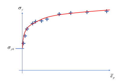
Figure 1. Parameter fitting of NLKIN or NLISO (demonstration)

Temperature-dependent combined hardening

If temperature-dependent combined hardening is active, then all the parameters are temperature dependent, for example,

C k ( T ) γ k ( T ) σ y 0 ( T ) Q ( T ) b ( T ) MathType@MTEF@5@5@+= feaagKart1ev2aaatCvAUfeBSjuyZL2yd9gzLbvyNv2CaerbuLwBLn hiov2DGi1BTfMBaeXatLxBI9gBaerbd9wDYLwzYbItLDharqqtubsr 4rNCHbGeaGqiVu0Je9sqqrpepC0xbbL8F4rqqrFfpeea0xe9Lq=Jc9 vqaqpepm0xbba9pwe9Q8fs0=yqaqpepae9pg0FirpepeKkFr0xfr=x fr=xb9adbaqaaeGaciGaaiaabeqaamaabaabaaGceaqabeaacaWGdb WaaSbaaSqaaiaadUgaaeqaaOGaaiikaiaadsfacaGGPaaabaGaeq4S dC2aaSbaaSqaaiaadUgaaeqaaOGaaiikaiaadsfacaGGPaaabaGaeq 4Wdm3aaSbaaSqaaiaadMhacaaIWaaabeaakiaacIcacaWGubGaaiyk aaqaaiaadgfacaGGOaGaamivaiaacMcaaeaacaWGIbGaaiikaiaads facaGGPaaaaaa@4B23@

From experiment is only possible to test a limited number of temperatures. Interpolation is used to solving for plasticity at a temperature in between the test temperatures.

Using isotropic hardening NLISO as an example, if the parameters are provided at two temperatures T 1 MathType@MTEF@5@5@+= feaagKart1ev2aaatCvAUfeBSjuyZL2yd9gzLbvyNv2CaerbuLwBLn hiov2DGi1BTfMBaeXatLxBI9gBaerbd9wDYLwzYbItLDharqqtubsr 4rNCHbGeaGqiVu0Je9sqqrpepC0xbbL8F4rqqrFfpeea0xe9Lq=Jc9 vqaqpepm0xbba9pwe9Q8fs0=yqaqpepae9pg0FirpepeKkFr0xfr=x fr=xb9adbaqaaeGaciGaaiaabeqaamaabaabaaGcbaGaamivamaaBa aaleaacaaIXaaabeaaaaa@37B6@ and T 2 MathType@MTEF@5@5@+= feaagKart1ev2aaatCvAUfeBSjuyZL2yd9gzLbvyNv2CaerbuLwBLn hiov2DGi1BTfMBaeXatLxBI9gBaerbd9wDYLwzYbItLDharqqtubsr 4rNCHbGeaGqiVu0Je9sqqrpepC0xbbL8F4rqqrFfpeea0xe9Lq=Jc9 vqaqpepm0xbba9pwe9Q8fs0=yqaqpepae9pg0FirpepeKkFr0xfr=x fr=xb9adbaqaaeGaciGaaiaabeqaamaabaabaaGcbaGaamivamaaBa aaleaacaaIXaaabeaaaaa@37B6@ , then there are two yield stress functions for interpolation:(7) σ y ( ε ¯ p , T 1 ) = σ y 0 + Q ( T 1 ) ( 1 e b ( T 1 ) ε ¯ p ) MathType@MTEF@5@5@+= feaagKart1ev2aaatCvAUfeBSjuyZL2yd9gzLbvyNv2CaerbuLwBLn hiov2DGi1BTfMBaeXatLxBI9gBaerbd9wDYLwzYbItLDharqqtubsr 4rNCHbGeaGqiVu0Je9sqqrpepC0xbbL8F4rqqrFfpeea0xe9Lq=Jc9 vqaqpepm0xbba9pwe9Q8fs0=yqaqpepae9pg0FirpepeKkFr0xfr=x fr=xb9adbaqaaeGaciGaaiaabeqaamaabaabaaGcbaGaeq4Wdm3aaS baaSqaaiaadMhaaeqaaOGaaiikaiqbew7aLzaaraWaaSbaaSqaaiaa dchaaeqaaOGaaiilaiaadsfadaWgaaWcbaGaaGymaaqabaGccaGGPa Gaeyypa0Jaeq4Wdm3aaSbaaSqaaiaadMhacaaIWaaabeaakiabgUca RiaadgfacaGGOaGaamivamaaBaaaleaacaaIXaaabeaakiaacMcacq GHflY1caGGOaGaaGymaiabgkHiTiaadwgadaahaaWcbeqaaiabgkHi TiaadkgacaGGOaGaamivamaaBaaameaacaaIXaaabeaaliaacMcacq GHflY1cuaH1oqzgaqeamaaBaaameaacaWGWbaabeaaaaGccaGGPaaa aa@59CC@ (8) σ y ( ε ¯ p , T 2 ) = σ y 0 + Q ( T 2 ) ( 1 e b ( T 2 ) ε ¯ p ) MathType@MTEF@5@5@+= feaagKart1ev2aaatCvAUfeBSjuyZL2yd9gzLbvyNv2CaerbuLwBLn hiov2DGi1BTfMBaeXatLxBI9gBaerbd9wDYLwzYbItLDharqqtubsr 4rNCHbGeaGqiVu0Je9sqqrpepC0xbbL8F4rqqrFfpeea0xe9Lq=Jc9 vqaqpepm0xbba9pwe9Q8fs0=yqaqpepae9pg0FirpepeKkFr0xfr=x fr=xb9adbaqaaeGaciGaaiaabeqaamaabaabaaGcbaGaeq4Wdm3aaS baaSqaaiaadMhaaeqaaOGaaiikaiqbew7aLzaaraWaaSbaaSqaaiaa dchaaeqaaOGaaiilaiaadsfadaWgaaWcbaGaaGOmaaqabaGccaGGPa Gaeyypa0Jaeq4Wdm3aaSbaaSqaaiaadMhacaaIWaaabeaakiabgUca RiaadgfacaGGOaGaamivamaaBaaaleaacaaIYaaabeaakiaacMcacq GHflY1caGGOaGaaGymaiabgkHiTiaadwgadaahaaWcbeqaaiabgkHi TiaadkgacaGGOaGaamivamaaBaaameaacaaIYaaabeaaliaacMcacq GHflY1cuaH1oqzgaqeamaaBaaameaacaWGWbaabeaaaaGccaGGPaaa aa@59CF@
The interpolated yield stress at the current temperature T c u r r MathType@MTEF@5@5@+= feaagKart1ev2aaatCvAUfeBSjuyZL2yd9gzLbvyNv2CaerbuLwBLn hiov2DGi1BTfMBaeXatLxBI9gBaerbd9wDYLwzYbItLDharqqtubsr 4rNCHbGeaGqiVu0Je9sqqrpepC0xbbL8F4rqqrFfpeea0xe9Lq=Jc9 vqaqpepm0xbba9pwe9Q8fs0=yqaqpepae9pg0FirpepeKkFr0xfr=x fr=xb9adbaqaaeGaciGaaiaabeqaamaabaabaaGcbaGaamivamaaBa aaleaacaWGJbGaamyDaiaadkhacaWGYbaabeaaaaa@3ACB@ in [ T 1 MathType@MTEF@5@5@+= feaagKart1ev2aaatCvAUfeBSjuyZL2yd9gzLbvyNv2CaerbuLwBLn hiov2DGi1BTfMBaeXatLxBI9gBaerbd9wDYLwzYbItLDharqqtubsr 4rNCHbGeaGqiVu0Je9sqqrpepC0xbbL8F4rqqrFfpeea0xe9Lq=Jc9 vqaqpepm0xbba9pwe9Q8fs0=yqaqpepae9pg0FirpepeKkFr0xfr=x fr=xb9adbaqaaeGaciGaaiaabeqaamaabaabaaGcbaGaamivamaaBa aaleaacaaIXaaabeaaaaa@37B6@ , T 2 MathType@MTEF@5@5@+= feaagKart1ev2aaatCvAUfeBSjuyZL2yd9gzLbvyNv2CaerbuLwBLn hiov2DGi1BTfMBaeXatLxBI9gBaerbd9wDYLwzYbItLDharqqtubsr 4rNCHbGeaGqiVu0Je9sqqrpepC0xbbL8F4rqqrFfpeea0xe9Lq=Jc9 vqaqpepm0xbba9pwe9Q8fs0=yqaqpepae9pg0FirpepeKkFr0xfr=x fr=xb9adbaqaaeGaciGaaiaabeqaamaabaabaaGcbaGaamivamaaBa aaleaacaaIXaaabeaaaaa@37B6@ ] is then,(9) σ y ( ε ¯ p , T c u r r ) = f 1 σ y ( ε ¯ p , T 1 ) + f 2 σ y ( ε ¯ p , T 2 ) MathType@MTEF@5@5@+= feaagKart1ev2aaatCvAUfeBSjuyZL2yd9gzLbvyNv2CaerbuLwBLn hiov2DGi1BTfMBaeXatLxBI9gBaerbd9wDYLwzYbItLDharqqtubsr 4rNCHbGeaGqiVu0Je9sqqrpepC0xbbL8F4rqqrFfpeea0xe9Lq=Jc9 vqaqpepm0xbba9pwe9Q8fs0=yqaqpepae9pg0FirpepeKkFr0xfr=x fr=xb9adbaqaaeGaciGaaiaabeqaamaabaabaaGcbaGaeq4Wdm3aaS baaSqaaiaadMhaaeqaaOGaaiikaiqbew7aLzaaraWaaSbaaSqaaiaa dchaaeqaaOGaaiilaiaadsfadaWgaaWcbaGaam4yaiaadwhacaWGYb GaamOCaaqabaGccaGGPaGaeyypa0JaamOzamaaBaaaleaacaaIXaaa beaakiabgwSixlabeo8aZnaaBaaaleaacaWG5baabeaakiaacIcacu aH1oqzgaqeamaaBaaaleaacaWGWbaabeaakiaacYcacaWGubWaaSba aSqaaiaaigdaaeqaaOGaaiykaiabgUcaRiaadAgadaWgaaWcbaGaaG OmaaqabaGccqGHflY1cqaHdpWCdaWgaaWcbaGaamyEaaqabaGccaGG OaGafqyTduMbaebadaWgaaWcbaGaamiCaaqabaGccaGGSaGaamivam aaBaaaleaacaaIYaaabeaakiaacMcaaaa@605D@

with two factors for different temperatures f 1 = T 2 T c u r r T 2 T 1 MathType@MTEF@5@5@+= feaagKart1ev2aaatCvAUfeBSjuyZL2yd9gzLbvyNv2CaerbuLwBLn hiov2DGi1BTfMBaeXatLxBI9gBaerbd9wDYLwzYbItLDharqqtubsr 4rNCHbGeaGqiVu0Je9sqqrpepC0xbbL8F4rqqrFfpeea0xe9Lq=Jc9 vqaqpepm0xbba9pwe9Q8fs0=yqaqpepae9pg0FirpepeKkFr0xfr=x fr=xb9adbaqaaeGaciGaaiaabeqaamaabaabaaGcbaGaamOzamaaBa aaleaacaaIXaaabeaakiabg2da9maalaaabaGaamivamaaBaaaleaa caaIYaaabeaakiabgkHiTiaadsfaqaaaaaaaaaWdbmaaBaaaleaaca WGJbGaamyDaiaadkhacaWGYbaabeaaaOWdaeaacaWGubWaaSbaaSqa aiaaikdaaeqaaOGaeyOeI0IaamivamaaBaaaleaacaaIXaaabeaaaa aaaa@4526@ , f 2 = T c u r r T 1 T 2 T 1 MathType@MTEF@5@5@+= feaagKart1ev2aaatCvAUfeBSjuyZL2yd9gzLbvyNv2CaerbuLwBLn hiov2DGi1BTfMBaeXatLxBI9gBaerbd9wDYLwzYbItLDharqqtubsr 4rNCHbGeaGqiVu0Je9sqqrpepC0xbbL8F4rqqrFfpeea0xe9Lq=Jc9 vqaqpepm0xbba9pwe9Q8fs0=yqaqpepae9pg0FirpepeKkFr0xfr=x fr=xb9adbaqaaeGaciGaaiaabeqaamaabaabaaGcbaGaamOzamaaBa aaleaacaaIYaaabeaakiabg2da9maalaaabaGaamivaabaaaaaaaaa peWaaSbaaSqaaiaadogacaWG1bGaamOCaiaadkhaaeqaaOWdaiabgk HiTiaadsfadaWgaaWcbaGaaGymaaqabaaakeaacaWGubWaaSbaaSqa aiaaikdaaeqaaOGaeyOeI0IaamivamaaBaaaleaacaaIXaaabeaaaa aaaa@4526@ .

As an example, Figure 2 illustrates the principle of interpolation.

It is worthy to mention that the parameters (Q and B) are not interpolated directly. Instead, the yield functions at two temperatures are interpolated. This is the similar case for NLKIN, where the evolution laws at two temperatures are interpolated.


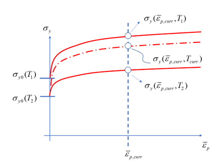
Figure 2. Principle of interpolation for temperature dependent NLISO

If the temperature, T MathType@MTEF@5@5@+= feaagKart1ev2aaatCvAUfeBSjuyZL2yd9gzLbvyNv2CaerbuLwBLn hiov2DGi1BTfMBaeXatLxBI9gBaerbd9wDYLwzYbItLDharqqtubsr 4rNCHbGeaGqiVu0Je9sqqrpepC0xbbL8F4rqqrFfpeea0xe9Lq=Jc9 vqaqpepm0xbba9pwe9Q8fs0=yqaqpepae9pg0FirpepeKkFr0xfr=x fr=xb9adbaqaaeGaciGaaiaabeqaamaabaabaaGcbaGaamivamaaBa aaleaacaaIXaaabeaaaaa@37B6@ is beyond the available temperature range [ T 1 MathType@MTEF@5@5@+= feaagKart1ev2aaatCvAUfeBSjuyZL2yd9gzLbvyNv2CaerbuLwBLn hiov2DGi1BTfMBaeXatLxBI9gBaerbd9wDYLwzYbItLDharqqtubsr 4rNCHbGeaGqiVu0Je9sqqrpepC0xbbL8F4rqqrFfpeea0xe9Lq=Jc9 vqaqpepm0xbba9pwe9Q8fs0=yqaqpepae9pg0FirpepeKkFr0xfr=x fr=xb9adbaqaaeGaciGaaiaabeqaamaabaabaaGcbaGaamivamaaBa aaleaacaaIXaaabeaaaaa@37B6@ , T 2 MathType@MTEF@5@5@+= feaagKart1ev2aaatCvAUfeBSjuyZL2yd9gzLbvyNv2CaerbuLwBLn hiov2DGi1BTfMBaeXatLxBI9gBaerbd9wDYLwzYbItLDharqqtubsr 4rNCHbGeaGqiVu0Je9sqqrpepC0xbbL8F4rqqrFfpeea0xe9Lq=Jc9 vqaqpepm0xbba9pwe9Q8fs0=yqaqpepae9pg0FirpepeKkFr0xfr=x fr=xb9adbaqaaeGaciGaaiaabeqaamaabaabaaGcbaGaamivamaaBa aaleaacaaIXaaabeaaaaa@37B6@ ], then closest temperature will be selected. In other words, no extrapolation of temperature is performed. Furthermore, it is suggested to provide the material parameter of NLKIN and NLISO at the same temperature.

Cast Iron Plasticity

Cast iron material model is used to describe the yield behavior of grey cast iron, in which tension and compression behavior are different.

In this material model, rate form is used for strain evolution and the strain rate is decomposed into two parts (elastic and plastic parts) in an additive way.(10) ε ˙ = ε ˙ e + ε ˙ p MathType@MTEF@5@5@+= feaagKart1ev2aqatCvAUfeBSjuyZL2yd9gzLbvyNv2CaerbuLwBLn hiov2DGi1BTfMBaeXatLxBI9gBaerbd9wDYLwzYbItLDharqqtubsr 4rNCHbGeaGqiVu0Je9sqqrpepC0xbbL8F4rqqrFfpeea0xe9Lq=Jc9 vqaqpepm0xbba9pwe9Q8fs0=yqaqpepae9pg0FirpepeKkFr0xfr=x fr=xb9adbaqaaeGaciGaaiaabeqaamaabaabaaGcbaGafqyTduMbai aacqGH9aqpcuaH1oqzgaGaamaaCaaaleqabaGaamyzaaaakiabgUca Riqbew7aLzaacaWaaWbaaSqabeaacaWGWbaaaaaa@3F32@

Yield Function

The yielding criteria is defined as:(11) f 0 MathType@MTEF@5@5@+= feaagKart1ev2aqatCvAUfeBSjuyZL2yd9gzLbvyNv2CaerbuLwBLn hiov2DGi1BTfMBaeXatLxBI9gBaerbd9wDYLwzYbItLDharqqtubsr 4rNCHbGeaGqiVu0Je9sqqrpepC0xbbL8F4rqqrFfpeea0xe9Lq=Jc9 vqaqpepm0xbba9pwe9Q8fs0=yqaqpepae9pg0FirpepeKkFr0xfr=x fr=xb9adbaqaaeGaciGaaiaabeqaamaabaabaaGcbaGaamOzaiabgs MiJkaaicdaaaa@3951@

Where,

f = { 2 3 q cos θ + p σ t     p > σ c 3 q σ c                       p σ c 3 MathType@MTEF@5@5@+= feaagKart1ev2aaatCvAUfeBSjuyZL2yd9gzLbvyNv2CaerbuLwBLn hiov2DGi1BTfMBaeXatLxBI9gBaerbd9wDYLwzYbItLDharqqtubsr 4rNCHbGeaGqiVu0Je9sqqrpepC0xbbL8F4rqqrFfpeea0xe9Lq=Jc9 vqaqpepm0xbba9pwe9Q8fs0=yqaqpepae9pg0FirpepeKkFr0xfr=x fr=xb9adbaqaaeGaciGaaiaabeqaamaabaabaaGcbaGaamOzaiabg2 da9maaceaabaqbaeqabiqaaaqaamaalaaabaGaaGOmaaqaaiaaioda aaGaamyCaiGacogacaGGVbGaai4CaiabeI7aXjabgUcaRiaadchacq GHsislcqaHdpWCdaWgaaWcbaGaamiDaaqabaGccaqGGaGaaeiiaiaa bccacaWGWbGaeyOpa4JaeyOeI0YaaSaaaeaacqaHdpWCdaWgaaWcba Gaam4yaaqabaaakeaacaaIZaaaaaqaaiaadghacqGHsislcqaHdpWC daWgaaWcbaGaam4yaaqabaGccaqGGaGaaeiiaiaabccacaqGGaGaae iiaiaabccacaqGGaGaaeiiaiaabccacaqGGaGaaeiiaiaabccacaqG GaGaaeiiaiaabccacaqGGaGaaeiiaiaabccacaqGGaGaaeiiaiaabc cacaWGWbGaeyizImQaeyOeI0YaaSaaaeaacqaHdpWCdaWgaaWcbaGa am4yaaqabaaakeaacaaIZaaaaaaaaiaawUhaaaaa@67B5@

The first criterion is Rankine criterion (max. Principal stress criterion) for tensile yielding, and the second criterion is von Mises criterion for compressive yielding. Together they form a composite yield surface.

Where,
σ t MathType@MTEF@5@5@+= feaagKart1ev2aaatCvAUfeBSjuyZL2yd9gzLbvyNv2CaerbuLwBLn hiov2DGi1BTfMBaeXatLxBI9gBaerbd9wDYLwzYbItLDharqqtubsr 4rNCHbGeaGqiVu0Je9sqqrpepC0xbbL8F4rqqrFfpeea0xe9Lq=Jc9 vqaqpepm0xbba9pwe9Q8fs0=yqaqpepae9pg0FirpepeKkFr0xfr=x fr=xb9adbaqaaeGaciGaaiaabeqaamaabaabaaGcbaGaeq4Wdm3aaS baaSqaaiaadshaaeqaaaaa@38DE@
Yield stress in uniaxial tension.
σ c MathType@MTEF@5@5@+= feaagKart1ev2aaatCvAUfeBSjuyZL2yd9gzLbvyNv2CaerbuLwBLn hiov2DGi1BTfMBaeXatLxBI9gBaerbd9wDYLwzYbItLDharqqtubsr 4rNCHbGeaGqiVu0Je9sqqrpepC0xbbL8F4rqqrFfpeea0xe9Lq=Jc9 vqaqpepm0xbba9pwe9Q8fs0=yqaqpepae9pg0FirpepeKkFr0xfr=x fr=xb9adbaqaaeGaciGaaiaabeqaamaabaabaaGcbaGaeq4Wdm3aaS baaSqaaiaadshaaeqaaaaa@38DE@
Yield stress in uniaxial compression.

Since the material is assumed to be isotropic, the yield surface can be expressed with a function of three invariant measure of the stress tensor, p MathType@MTEF@5@5@+= feaagKart1ev2aaatCvAUfeBSjuyZL2yd9gzLbvyNv2CaerbuLwBLn hiov2DGi1BTfMBaeXatLxBI9gBaerbd9wDYLwzYbItLDharqqtubsr 4rNCHbGeaGqiVu0Je9sqqrpepC0xbbL8F4rqqrFfpeea0xe9Lq=Jc9 vqaqpepm0xbba9pwe9Q8fs0=yqaqpepae9pg0FirpepeKkFr0xfr=x fr=xb9adbaqaaeGaciGaaiaabeqaamaabaabaaGcbaGaamiCaaaa@36EB@ , q MathType@MTEF@5@5@+= feaagKart1ev2aaatCvAUfeBSjuyZL2yd9gzLbvyNv2CaerbuLwBLn hiov2DGi1BTfMBaeXatLxBI9gBaerbd9wDYLwzYbItLDharqqtubsr 4rNCHbGeaGqiVu0Je9sqqrpepC0xbbL8F4rqqrFfpeea0xe9Lq=Jc9 vqaqpepm0xbba9pwe9Q8fs0=yqaqpepae9pg0FirpepeKkFr0xfr=x fr=xb9adbaqaaeGaciGaaiaabeqaamaabaabaaGcbaGaamiCaaaa@36EB@ , and r MathType@MTEF@5@5@+= feaagKart1ev2aaatCvAUfeBSjuyZL2yd9gzLbvyNv2CaerbuLwBLn hiov2DGi1BTfMBaeXatLxBI9gBaerbd9wDYLwzYbItLDharqqtubsr 4rNCHbGeaGqiVu0Je9sqqrpepC0xbbL8F4rqqrFfpeea0xe9Lq=Jc9 vqaqpepm0xbba9pwe9Q8fs0=yqaqpepae9pg0FirpepeKkFr0xfr=x fr=xb9adbaqaaeGaciGaaiaabeqaamaabaabaaGcbaGaamiCaaaa@36EB@ .

Where, q MathType@MTEF@5@5@+= feaagKart1ev2aaatCvAUfeBSjuyZL2yd9gzLbvyNv2CaerbuLwBLn hiov2DGi1BTfMBaeXatLxBI9gBaerbd9wDYLwzYbItLDharqqtubsr 4rNCHbGeaGqiVu0Je9sqqrpepC0xbbL8F4rqqrFfpeea0xe9Lq=Jc9 vqaqpepm0xbba9pwe9Q8fs0=yqaqpepae9pg0FirpepeKkFr0xfr=x fr=xb9adbaqaaeGaciGaaiaabeqaamaabaabaaGcbaGaamiCaaaa@36EB@ is von Mises stress of a given stress state.(12) q = 3 J 2 = 3 2 S : S MathType@MTEF@5@5@+= feaagKart1ev2aqatCvAUfeBSjuyZL2yd9gzLbvyNv2CaerbuLwBLn hiov2DGi1BTfMBaeXatLxBI9gBaerbd9wDYLwzYbItLDharqqtubsr 4rNCHbGeaGqiVu0Je9sqqrpepC0xbbL8F4rqqrFfpeea0xe9Lq=Jc9 vqaqpepm0xbba9pwe9Q8fs0=yqaqpepae9pg0FirpepeKkFr0xfr=x fr=xb9adbaqaaeGaciGaaiaabeqaamaabaabaaGcbaGaamyCaiabg2 da9maakaaabaGaaG4maiaadQeadaWgaaWcbaGaaGOmaaqabaaabeaa kiabg2da9maakaaabaWaaSaaaeaacaaIZaaabaGaaGOmaaaacaWHtb GaaiOoaiaahofaaSqabaaaaa@3FA1@
Where, p MathType@MTEF@5@5@+= feaagKart1ev2aaatCvAUfeBSjuyZL2yd9gzLbvyNv2CaerbuLwBLn hiov2DGi1BTfMBaeXatLxBI9gBaerbd9wDYLwzYbItLDharqqtubsr 4rNCHbGeaGqiVu0Je9sqqrpepC0xbbL8F4rqqrFfpeea0xe9Lq=Jc9 vqaqpepm0xbba9pwe9Q8fs0=yqaqpepae9pg0FirpepeKkFr0xfr=x fr=xb9adbaqaaeGaciGaaiaabeqaamaabaabaaGcbaGaamiCaaaa@36EB@ is mean stress given by:(13) p = σ x x + σ y y + σ z z 3 MathType@MTEF@5@5@+= feaagKart1ev2aqatCvAUfeBSjuyZL2yd9gzLbvyNv2CaerbuLwBLn hiov2DGi1BTfMBaeXatLxBI9gBaerbd9wDYLwzYbItLDharqqtubsr 4rNCHbGeaGqiVu0Je9sqqrpepC0xbbL8F4rqqrFfpeea0xe9Lq=Jc9 vqaqpepm0xbba9pwe9Q8fs0=yqaqpepae9pg0FirpepeKkFr0xfr=x fr=xb9adbaqaaeGaciGaaiaabeqaamaabaabaaGcbaGaamiCaiabg2 da9maalaaabaGaeq4Wdm3aaSbaaSqaaiaadIhacaWG4baabeaakiab gUcaRiabeo8aZnaaBaaaleaacaWG5bGaamyEaaqabaGccqGHRaWkcq aHdpWCdaWgaaWcbaGaamOEaiaadQhaaeqaaaGcbaGaaG4maaaaaaa@4662@
The invariant r MathType@MTEF@5@5@+= feaagKart1ev2aaatCvAUfeBSjuyZL2yd9gzLbvyNv2CaerbuLwBLn hiov2DGi1BTfMBaeXatLxBI9gBaerbd9wDYLwzYbItLDharqqtubsr 4rNCHbGeaGqiVu0Je9sqqrpepC0xbbL8F4rqqrFfpeea0xe9Lq=Jc9 vqaqpepm0xbba9pwe9Q8fs0=yqaqpepae9pg0FirpepeKkFr0xfr=x fr=xb9adbaqaaeGaciGaaiaabeqaamaabaabaaGcbaGaamiCaaaa@36EB@ can be expressed as:(14) r = ( 9 2 S · S : S ) 1 3 MathType@MTEF@5@5@+= feaagKart1ev2aaatCvAUfeBSjuyZL2yd9gzLbvyNv2CaerbuLwBLn hiov2DGi1BTfMBaeXatLxBI9gBaerbd9wDYLwzYbItLDharqqtubsr 4rNCHbGeaGqiVu0Je9sqqrpepC0xbbL8F4rqqrFfpeea0xe9Lq=Jc9 vqaqpepm0xbba9pwe9Q8fs0=yqaqpepae9pg0FirpepeKkFr0xfr=x fr=xb9adbaqaaeGaciGaaiaabeqaamaabaabaaGcbaGaamOCaiabg2 da9maabmaabaWaaSaaaeaacaaI5aaabaGaaGOmaaaacaWHtbGaeS4J PFMaaC4uaiaacQdacaWHtbaacaGLOaGaayzkaaWaaWbaaSqabeaada WcaaqaaiaaigdaaeaacaaIZaaaaaaaaaa@4282@
Where, S MathType@MTEF@5@5@+= feaagKart1ev2aqatCvAUfeBSjuyZL2yd9gzLbvyNv2CaerbuLwBLn hiov2DGi1BTfMBaeXatLxBI9gBaerbd9wDYLwzYbItLDharqqtubsr 4rNCHbGeaGqiVu0Je9sqqrpepC0xbbL8F4rqqrFfpeea0xe9Lq=Jc9 vqaqpepm0xbba9pwe9Q8fs0=yqaqpepae9pg0FirpepeKkFr0xfr=x fr=xb9adbaqaaeGaciGaaiaabeqaamaabaabaaGcbaGaaC4uaaaa@36D3@ is the tensor form of deviatoric stress.(15) S = [ S x x S x y S x z S y x S y y S y z S z x S z y S z z ] MathType@MTEF@5@5@+= feaagKart1ev2aqatCvAUfeBSjuyZL2yd9gzLbvyNv2CaerbuLwBLn hiov2DGi1BTfMBaeXatLxBI9gBaerbd9wDYLwzYbItLDharqqtubsr 4rNCHbGeaGqiVu0Je9sqqrpepC0xbbL8F4rqqrFfpeea0xe9Lq=Jc9 vqaqpepm0xbba9pwe9Q8fs0=yqaqpepae9pg0FirpepeKkFr0xfr=x fr=xb9adbaqaaeGaciGaaiaabeqaamaabaabaaGcbaGaaC4uaiabg2 da9maadmaabaqbaeqabmWaaaqaaiaadofadaWgaaWcbaGaamiEaiaa dIhaaeqaaaGcbaGaam4uamaaBaaaleaacaWG4bGaamyEaaqabaaake aacaWGtbWaaSbaaSqaaiaadIhacaWG6baabeaaaOqaaiaadofadaWg aaWcbaGaamyEaiaadIhaaeqaaaGcbaGaam4uamaaBaaaleaacaWG5b GaamyEaaqabaaakeaacaWGtbWaaSbaaSqaaiaadMhacaWG6baabeaa aOqaaiaadofadaWgaaWcbaGaamOEaiaadIhaaeqaaaGcbaGaam4uam aaBaaaleaacaWG6bGaamyEaaqabaaakeaacaWGtbWaaSbaaSqaaiaa dQhacaWG6baabeaaaaaakiaawUfacaGLDbaaaaa@553C@
The quantity θ is Lode’s Angle that is defined by q MathType@MTEF@5@5@+= feaagKart1ev2aaatCvAUfeBSjuyZL2yd9gzLbvyNv2CaerbuLwBLn hiov2DGi1BTfMBaeXatLxBI9gBaerbd9wDYLwzYbItLDharqqtubsr 4rNCHbGeaGqiVu0Je9sqqrpepC0xbbL8F4rqqrFfpeea0xe9Lq=Jc9 vqaqpepm0xbba9pwe9Q8fs0=yqaqpepae9pg0FirpepeKkFr0xfr=x fr=xb9adbaqaaeGaciGaaiaabeqaamaabaabaaGcbaGaamiCaaaa@36EB@ and r MathType@MTEF@5@5@+= feaagKart1ev2aaatCvAUfeBSjuyZL2yd9gzLbvyNv2CaerbuLwBLn hiov2DGi1BTfMBaeXatLxBI9gBaerbd9wDYLwzYbItLDharqqtubsr 4rNCHbGeaGqiVu0Je9sqqrpepC0xbbL8F4rqqrFfpeea0xe9Lq=Jc9 vqaqpepm0xbba9pwe9Q8fs0=yqaqpepae9pg0FirpepeKkFr0xfr=x fr=xb9adbaqaaeGaciGaaiaabeqaamaabaabaaGcbaGaamiCaaaa@36EB@ as shown below, which identifies the meridional plane for a given stress state.(16) cos ( 3 θ ) = ( r q ) 3 MathType@MTEF@5@5@+= feaagKart1ev2aqatCvAUfeBSjuyZL2yd9gzLbvyNv2CaerbuLwBLn hiov2DGi1BTfMBaeXatLxBI9gBaerbd9wDYLwzYbItLDharqqtubsr 4rNCHbGeaGqiVu0Je9sqqrpepC0xbbL8F4rqqrFfpeea0xe9Lq=Jc9 vqaqpepm0xbba9pwe9Q8fs0=yqaqpepae9pg0FirpepeKkFr0xfr=x fr=xb9adbaqaaeGaciGaaiaabeqaamaabaabaaGcbaGaci4yaiaac+ gacaGGZbWaaeWaaeaacaaIZaGaeqiUdehacaGLOaGaayzkaaGaeyyp a0ZaaeWaaeaadaWcaaqaaiaadkhaaeaacaWGXbaaaaGaayjkaiaawM caamaaCaaaleqabaGaaG4maaaaaaa@423C@

In the principal stress space, the yield function is a von Mises cylinder intersected with Rankine planes (Figure 3). The yield surface is illustrated in π MathType@MTEF@5@5@+= feaagKart1ev2aaatCvAUfeBSjuyZL2yd9gzLbvyNv2CaerbuLwBLn hiov2DGi1BTfMBaeXatLxBI9gBaerbd9wDYLwzYbItLDharqqtubsr 4rNCHbGeaGqiVu0Je9sqqrpepC0xbbL8F4rqqrFfpeea0xe9Lq=Jc9 vqaqpepm0xbba9pwe9Q8fs0=yqaqpepae9pg0FirpepeKkFr0xfr=x fr=xb9adbaqaaeGaciGaaiaabeqaamaabaabaaGcbaGaeqiWdahaaa@37B3@ plane in Figure 4 and Figure 5, and in meridional plane in Figure 6.

(17) r = ( 9 2 S S : S ) MathType@MTEF@5@5@+= feaagKart1ev2aqatCvAUfeBSjuyZL2yd9gzLbvyNv2CaerbuLwBLn hiov2DGi1BTfMBaeXatLxBI9gBaerbd9wDYLwzYbItLDharqqtubsr 4rNCHbGeaGqiVu0Je9sqqrpepC0xbbL8F4rqqrFfpeea0xe9Lq=Jc9 vqaqpepm0xbba9pwe9Q8fs0=yqaqpepae9pg0FirpepeKkFr0xfr=x fr=xb9adbaqaaeGaciGaaiaabeqaamaabaabaaGcbaGaamOCaiabg2 da9maabmaabaWaaSaaaeaacaaI5aaabaGaaGOmaaaacaWHtbGaeyyX ICTaaC4uaiaacQdacaWHtbaacaGLOaGaayzkaaaaaa@40A8@

Where, S MathType@MTEF@5@5@+= feaagKart1ev2aqatCvAUfeBSjuyZL2yd9gzLbvyNv2CaerbuLwBLn hiov2DGi1BTfMBaeXatLxBI9gBaerbd9wDYLwzYbItLDharqqtubsr 4rNCHbGeaGqiVu0Je9sqqrpepC0xbbL8F4rqqrFfpeea0xe9Lq=Jc9 vqaqpepm0xbba9pwe9Q8fs0=yqaqpepae9pg0FirpepeKkFr0xfr=x fr=xb9adbaqaaeGaciGaaiaabeqaamaabaabaaGcbaGaaC4uaaaa@36D3@ is the tensor form of deviatoric stress.

Yield Surface of cast iron plasticity.


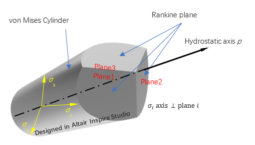
Figure 3. Overview on the yield surface


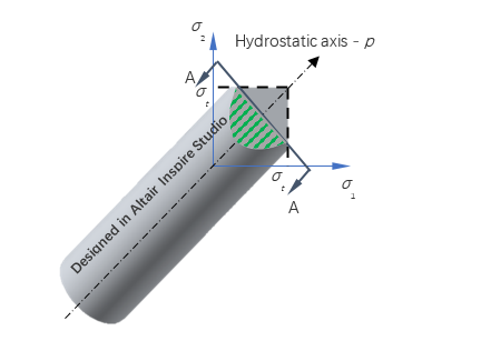
Figure 4. σ1-σ2 plane view


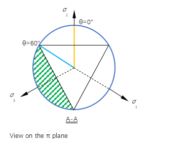
Figure 5. A-A view on the π plane


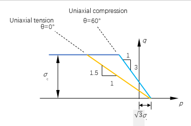
Figure 6. Meridional plane view

Flow Rule

The flow rule is expressed as:(18) { ( p g ) 2 a 2 + q 2 = 9 g 2      p > σ c 3 q = 3 g                          p σ c 3     MathType@MTEF@5@5@+= feaagKart1ev2aaatCvAUfeBSjuyZL2yd9gzLbvyNv2CaerbuLwBLn hiov2DGi1BTfMBaeXatLxBI9gBaerbd9wDYLwzYbItLDharqqtubsr 4rNCHbGeaGqiVu0Je9sqqrpepC0xbbL8F4rqqrFfpeea0xe9Lq=Jc9 vqaqpepm0xbba9pwe9Q8fs0=yqaqpepae9pg0FirpepeKkFr0xfr=x fr=xb9adbaqaaeGaciGaaiaabeqaamaabaabaaGcbaWaaiqaaeaafa qabeGabaaabaWaaSaaaeaadaqadaqaaiaadchacqGHsislcaWGNbaa caGLOaGaayzkaaWaaWbaaSqabeaacaaIYaaaaaGcbaGaamyyamaaCa aaleqabaGaaGOmaaaaaaGccqGHRaWkcaWGXbWaaWbaaSqabeaacaaI YaaaaOGaeyypa0JaaGyoaiaadEgadaahaaWcbeqaaiaaikdaaaGcca qGGaGaaeiiaiaabccacaqGGaGaamiCaiabg6da+iabgkHiTmaalaaa baGaeq4Wdm3aaSbaaSqaaiaadogaaeqaaaGcbaGaaG4maaaaaeaaca WGXbGaeyypa0JaaG4maiaadEgacaqGGaGaaeiiaiaabccacaqGGaGa aeiiaiaabccacaqGGaGaaeiiaiaabccacaqGGaGaaeiiaiaabccaca qGGaGaaeiiaiaabccacaqGGaGaaeiiaiaabccacaqGGaGaaeiiaiaa bccacaqGGaGaaeiiaiaabccacaWGWbGaeyizImQaeyOeI0YaaSaaae aacqaHdpWCdaWgaaWcbaGaam4yaaqabaaakeaacaaIZaaaaaaaaiaa wUhaaiaabccacaqGGaGaaeiiaaaa@6A02@

Hardening Rule

In this material model, only isotropic hardening is considered. The yield strength is increasing as the equivalent plastic strain grows. It is noted that as tension and the compression have different flow rules, the equivalent plastic strain is different for tension and compression. Hence, the tensile yield strength and the compressive yield strength are looked up from the tensile and the compressive table separately.

The compressive equivalent plastic strain is expressed as:(19) e n plc = e n1 plc + e ˙ plc MathType@MTEF@5@5@+= feaagKart1ev2aqatCvAUfeBSjuyZL2yd9gzLbvyNv2CaerbuLwBLn hiov2DGi1BTfMBaeXatLxBI9gBaerbd9wDYLwzYbItLDharqqtubsr 4rNCHbGeaGqiVu0Je9sqqrpepC0xbbL8F4rqqrFfpeea0xe9Lq=Jc9 vqaqpepm0xbba9pwe9Q8fs0=yqaqpepae9pg0FirpepeKkFr0xfr=x fr=xb9adbaqaaeGaciGaaiaabeqaamaabaabaaGcbaGaamyzamaaDa aaleaacaWGUbaabaGaamiCaiaadYgacaWGJbaaaOGaeyypa0Jaamyz amaaDaaaleaacaWGUbGaeyOeI0IaaGymaaqaaiaadchacaWGSbGaam 4yaaaakiabgUcaRiqadwgagaGaamaaCaaaleqabaGaamiCaiaadYga caWGJbaaaaaa@4739@ (20) e ˙ plc = 2 3 S( ε ˙ p ):S( ε ˙ p ) MathType@MTEF@5@5@+= feaagKart1ev2aqatCvAUfeBSjuyZL2yd9gzLbvyNv2CaerbuLwBLn hiov2DGi1BTfMBaeXatLxBI9gBaerbd9wDYLwzYbItLDharqqtubsr 4rNCHbGeaGqiVu0Je9sqqrpepC0xbbL8F4rqqrFfpeea0xe9Lq=Jc9 vqaqpepm0xbba9pwe9Q8fs0=yqaqpepae9pg0FirpepeKkFr0xfr=x fr=xb9adbaqaaeGaciGaaiaabeqaamaabaabaaGcbaGabmyzayaaca WaaWbaaSqabeaacaWGWbGaamiBaiaadogaaaGccqGH9aqpdaGcaaqa amaalaaabaGaaGOmaaqaaiaaiodaaaGaaC4uamaabmaabaGafqyTdu MbaiaadaahaaWcbeqaaiaadchaaaaakiaawIcacaGLPaaacaGG6aGa aC4uamaabmaabaGafqyTduMbaiaadaahaaWcbeqaaiaadchaaaaaki aawIcacaGLPaaaaSqabaaaaa@47D9@

Where, S( ε ˙ p ) MathType@MTEF@5@5@+= feaagKart1ev2aqatCvAUfeBSjuyZL2yd9gzLbvyNv2CaerbuLwBLn hiov2DGi1BTfMBaeXatLxBI9gBaerbd9wDYLwzYbItLDharqqtubsr 4rNCHbGeaGqiVu0Je9sqqrpepC0xbbL8F4rqqrFfpeea0xe9Lq=Jc9 vqaqpepm0xbba9pwe9Q8fs0=yqaqpepae9pg0FirpepeKkFr0xfr=x fr=xb9adbaqaaeGaciGaaiaabeqaamaabaabaaGcbaGaaC4uamaabm aabaGafqyTduMbaiaadaahaaWcbeqaaiaadchaaaaakiaawIcacaGL Paaaaaa@3B38@ is the tensor of deviatoric part of plastic strain rate.

The tensile equivalent plastic strain is:(21) e n plt = e n1 plt + e ˙ plt MathType@MTEF@5@5@+= feaagKart1ev2aqatCvAUfeBSjuyZL2yd9gzLbvyNv2CaerbuLwBLn hiov2DGi1BTfMBaeXatLxBI9gBaerbd9wDYLwzYbItLDharqqtubsr 4rNCHbGeaGqiVu0Je9sqqrpepC0xbbL8F4rqqrFfpeea0xe9Lq=Jc9 vqaqpepm0xbba9pwe9Q8fs0=yqaqpepae9pg0FirpepeKkFr0xfr=x fr=xb9adbaqaaeGaciGaaiaabeqaamaabaabaaGcbaGaamyzamaaDa aaleaacaWGUbaabaGaamiCaiaadYgacaWG0baaaOGaeyypa0Jaamyz amaaDaaaleaacaWGUbGaeyOeI0IaaGymaaqaaiaadchacaWGSbGaam iDaaaakiabgUcaRiqadwgagaGaamaaCaaaleqabaGaamiCaiaadYga caWG0baaaaaa@476C@ (22) e ˙ plc = 1 σ tn ( p ε ˙ vol p +q e ˙ plc ) MathType@MTEF@5@5@+= feaagKart1ev2aqatCvAUfeBSjuyZL2yd9gzLbvyNv2CaerbuLwBLn hiov2DGi1BTfMBaeXatLxBI9gBaerbd9wDYLwzYbItLDharqqtubsr 4rNCHbGeaGqiVu0Je9sqqrpepC0xbbL8F4rqqrFfpeea0xe9Lq=Jc9 vqaqpepm0xbba9pwe9Q8fs0=yqaqpepae9pg0FirpepeKkFr0xfr=x fr=xb9adbaqaaeGaciGaaiaabeqaamaabaabaaGcbaGabmyzayaaca WaaWbaaSqabeaacaWGWbGaamiBaiaadogaaaGccqGH9aqpdaWcaaqa aiaaigdaaeaacqaHdpWCdaWgaaWcbaGaamiDaiaad6gaaeqaaaaakm aabmaabaGaamiCaiqbew7aLzaacaWaa0baaSqaaiaadAhacaWGVbGa amiBaaqaaiaadchaaaGccqGHRaWkcaWGXbGabmyzayaacaWaaWbaaS qabeaacaWGWbGaamiBaiaadogaaaaakiaawIcacaGLPaaaaaa@4DAF@

Where, ε ˙ vol p = ε ˙ xx p + ε ˙ yy p + ε ˙ zz p MathType@MTEF@5@5@+= feaagKart1ev2aqatCvAUfeBSjuyZL2yd9gzLbvyNv2CaerbuLwBLn hiov2DGi1BTfMBaeXatLxBI9gBaerbd9wDYLwzYbItLDharqqtubsr 4rNCHbGeaGqiVu0Je9sqqrpepC0xbbL8F4rqqrFfpeea0xe9Lq=Jc9 vqaqpepm0xbba9pwe9Q8fs0=yqaqpepae9pg0FirpepeKkFr0xfr=x fr=xb9adbaqaaeGaciGaaiaabeqaamaabaabaaGcbaGafqyTduMbai aadaqhaaWcbaGaamODaiaad+gacaWGSbaabaGaamiCaaaakiabg2da 9iqbew7aLzaacaWaa0baaSqaaiaadIhacaWG4baabaGaamiCaaaaki abgUcaRiqbew7aLzaacaWaa0baaSqaaiaadMhacaWG5baabaGaamiC aaaakiabgUcaRiqbew7aLzaacaWaa0baaSqaaiaadQhacaWG6baaba GaamiCaaaaaaa@4CFB@ .

In the above expressions, the subscript index n MathType@MTEF@5@5@+= feaagKart1ev2aqatCvAUfeBSjuyZL2yd9gzLbvyNv2CaerbuLwBLn hiov2DGi1BTfMBaeXatLxBI9gBaerbd9wDYLwzYbItLDharqqtubsr 4rNCHbGeaGqiVu0Je9sqqrpepC0xbbL8F4rqqrFfpeea0xe9Lq=Jc9 vqaqpepm0xbba9pwe9Q8fs0=yqaqpepae9pg0FirpepeKkFr0xfr=x fr=xb9adbaqaaeGaciGaaiaabeqaamaabaabaaWcbaGaamOBaaaa@36EB@ implies the physical quantity is at time t = n MathType@MTEF@5@5@+= feaagKart1ev2aqatCvAUfeBSjuyZL2yd9gzLbvyNv2CaerbuLwBLn hiov2DGi1BTfMBaeXatLxBI9gBaerbd9wDYLwzYbItLDharqqtubsr 4rNCHbGeaGqiVu0Je9sqqrpepC0xbbL8F4rqqrFfpeea0xe9Lq=Jc9 vqaqpepm0xbba9pwe9Q8fs0=yqaqpepae9pg0FirpepeKkFr0xfr=x fr=xb9adbaqaaeGaciGaaiaabeqaamaabaabaaGcbaWccaWG0bGaey ypa0JaamOBaaaa@38F4@ , and n 1 MathType@MTEF@5@5@+= feaagKart1ev2aqatCvAUfeBSjuyZL2yd9gzLbvyNv2CaerbuLwBLn hiov2DGi1BTfMBaeXatLxBI9gBaerbd9wDYLwzYbItLDharqqtubsr 4rNCHbGeaGqiVu0Je9sqqrpepC0xbbL8F4rqqrFfpeea0xe9Lq=Jc9 vqaqpepm0xbba9pwe9Q8fs0=yqaqpepae9pg0FirpepeKkFr0xfr=x fr=xb9adbaqaaeGaciGaaiaabeqaamaabaabaaWcbaGaamOBaiabgk HiTiaaigdaaaa@3893@ means the physical quantity is at the last converged time t = n 1 MathType@MTEF@5@5@+= feaagKart1ev2aqatCvAUfeBSjuyZL2yd9gzLbvyNv2CaerbuLwBLn hiov2DGi1BTfMBaeXatLxBI9gBaerbd9wDYLwzYbItLDharqqtubsr 4rNCHbGeaGqiVu0Je9sqqrpepC0xbbL8F4rqqrFfpeea0xe9Lq=Jc9 vqaqpepm0xbba9pwe9Q8fs0=yqaqpepae9pg0FirpepeKkFr0xfr=x fr=xb9adbaqaaeGaciGaaiaabeqaamaabaabaaGcbaWccaWG0bGaey ypa0JaamOBaiabgkHiTiaaigdaaaa@3A9C@ .

Input

Cast iron plasticity material data can be specified by using the MCIRON Bulk Data Entry which has the same identification number as an existing MAT1 Bulk Data Entry. The Tensile and Compressive stress-strain curves can be defined using the TABLE_T and TABLE_C fields on the MCIRON entry.

Cast iron material via MCIRON is supported for Small and Large Displacement Nonlinear Static Analysis and Nonlinear Transient Analysis. It is supported for CHEXA, CTETRA, CPENTA, and CPYRA elements (both first and second order).

In addition to regular result output, additional results from this material model are output if STRAIN(PLASTIC) I/O Option is specified. These results include, 6 plastic strain components, equivalent compressive plastic strain, equivalent tensile plastic strain, nodal results, and integration results are also available.

Multiscale Modeling

OptiStruct (OS) and Multiscale Designer (MDS) can be combined to perform multiscaling analysis on structural components utilizing both linear and nonlinear materials.

Heterogeneous materials such as composites, soil, solid foams, and polycrystals consist of one or more distinguishable constituents that have different mechanical properties. 12 For example, it is known that fiber-reinforced composite materials have a stiffer and stronger phase known as the reinforcement and, a less stiff and weaker phase known as the matrix. The governing equations are well understood in one of the scales, either the micro-scale or the macro-scale. While general constitutive equations are applicable to solids under deformation in the macro-scale, continuum models are required in the micro-scale. In order to bridge the gap between the two scales, you need to consider models at different scales simultaneously. This can be achieved by multiscaling techniques.

Classical laminate theory can predict the overall properties of heterogeneous laminates; whereas, homogenization theory provides information on the individual phase properties and phase geometries. Knowledge of individual phases is important to characterize material damage and failure. Hence, multiscaling techniques open unique opportunities for modeling by focusing the material behavior on different levels of physical laws.

An overall flowchart for integration between the two softwares is provided in Figure 7. Multiscale Designer has four pre-processing steps which are used to create material subroutines. These subroutines characterize the micro-scale material behavior in the linear and nonlinear domain. Later they are integrated with OptiStruct through the MATUSR material card for structural analysis.


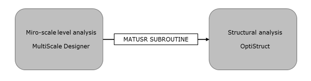
Figure 7. Multiscale Designer - OptiStruct Integration
The four pre-processing steps in Multiscale Designer are:
  1. Unit cell geometry and mesh definition
  2. Linear material characterization
  3. Reduced-order homogenization
  4. Nonlinear material characterization
Note: Detailed information on the four pre-processing steps is explained in the Multiscale Designer User Manual. 10 Users are expected to understand material characterization in Multiscale Designer.

Single-scale Model

The basic steps required to construct a single-scale material model.

Cast iron plasticity is interesting to study because it has different yielding and hardening behavior when subjected to tensile and compressive loads. The first two sections explain the input data required from the Multiscale Designer (MDS). The next two sections explain the procedure to integrate the material in OptiStruct (OS) and perform structural analysis.

Linear Material Characterization

The material model type is selected as a single scale material characterization. Multiscale Designer allows material characterization for:
  • isotropic
  • trans-isotopic
  • orthotropic
  • anisotropic material

Here a homogeneous material with the properties of cast iron is utilized for characterization in the linear regime. The input elastic properties/parameters and values of the material are:

Linear elastic parameter properties and values of cast iron 11
Tensile Young’s modulus (GPa), E t MathType@MTEF@5@5@+= feaagKart1ev2aqatCvAUfeBSjuyZL2yd9gzLbvyNv2CaerbuLwBLn hiov2DGi1BTfMBaeXatLxBI9gBaerbd9wDYLwzYbItLDharqqtubsr 4rNCHbGeaGqiVCI8FfYJH8YrFfeuY=Hhbbf9v8qqaqFr0xc9pk0xbb a9q8WqFfeaY=biLkVcLq=JHqpepeea0=as0Fb9pgeaYRXxe9vr0=vr 0=vqpWqaaeaabiGaciaacaqabeaadaqaaqaaaOqaaabaaaaaaaaape Gaamyra8aadaWgaaWcbaWdbiaadshaa8aabeaaaaa@3829@
95.5
Compressive Young’s modulus (GPa), E c MathType@MTEF@5@5@+= feaagKart1ev2aqatCvAUfeBSjuyZL2yd9gzLbvyNv2CaerbuLwBLn hiov2DGi1BTfMBaeXatLxBI9gBaerbd9wDYLwzYbItLDharqqtubsr 4rNCHbGeaGqiVCI8FfYJH8YrFfeuY=Hhbbf9v8qqaqFr0xc9pk0xbb a9q8WqFfeaY=biLkVcLq=JHqpepeea0=as0Fb9pgeaYRXxe9vr0=vr 0=vqpWqaaeaabiGaciaacaqabeaadaqaaqaaaOqaaabaaaaaaaaape Gaamyra8aadaWgaaWcbaWdbiaadshaa8aabeaaaaa@3829@
95.5
Poisson's ratio, ν MathType@MTEF@5@5@+= feaagKart1ev2aqatCvAUfeBSjuyZL2yd9gzLbvyNv2CaerbuLwBLn hiov2DGi1BTfMBaeXatLxBI9gBaerbd9wDYLwzYbItLDharqqtubsr 4rNCHbGeaGqiVCI8FfYJH8YrFfeuY=Hhbbf9v8qqaqFr0xc9pk0xbb a9q8WqFfeaY=biLkVcLq=JHqpepeea0=as0Fb9pgeaYRXxe9vr0=vr 0=vqpWqaaeaabiGaciaacaqabeaadaqaaqaaaOqaaabaaaaaaaaape GaeqyVd4gaaa@37C4@
0.26

Nonlinear Material Characterization

Various constitutive laws are available in Multiscale Designer, such as rate-independent plasticity, visco-elasticity, damage laws. Here isotropic damage – 3-piecewise Linear Evolution is used to simulate the nonlinear behavior of the material. The damage model formulation within Multiscale Designer follows the continuum damage mechanics framework. The elastic stiffness matrix is degraded by using a damage state variable which is a function of principal strains. Only for compressive loads, the principal strains are multiplied by a compression factor to alleviate the damage in compression. The compression factor is calculated internally, based on the input properties of the material.

Failure input parameter properties and values of cast iron 11
Stress at damage initiation – tension (MPa), σ 0 MathType@MTEF@5@5@+= feaagKart1ev2aqatCvAUfeBSjuyZL2yd9gzLbvyNv2CaerbuLwBLn hiov2DGi1BTfMBaeXatLxBI9gBaerbd9wDYLwzYbItLDharqqtubsr 4rNCHbGeaGqiVCI8FfYJH8YrFfeuY=Hhbbf9v8qqaqFr0xc9pk0xbb a9q8WqFfeaY=biLkVcLq=JHqpepeea0=as0Fb9pgeaYRXxe9vr0=vr 0=vqpWqaaeaabiGaciaacaqabeaadaqaaqaaaOqaaabaaaaaaaaape Gaeq4Wdm3damaaCaaaleqabaWdbiaaicdaaaaaaa@38D5@
126.0
Ultimate stress – tension (MPa), σ 1 MathType@MTEF@5@5@+= feaagKart1ev2aqatCvAUfeBSjuyZL2yd9gzLbvyNv2CaerbuLwBLn hiov2DGi1BTfMBaeXatLxBI9gBaerbd9wDYLwzYbItLDharqqtubsr 4rNCHbGeaGqiVCI8FfYJH8YrFfeuY=Hhbbf9v8qqaqFr0xc9pk0xbb a9q8WqFfeaY=biLkVcLq=JHqpepeea0=as0Fb9pgeaYRXxe9vr0=vr 0=vqpWqaaeaabiGaciaacaqabeaadaqaaqaaaOqaaabaaaaaaaaape Gaeq4Wdm3damaaCaaaleqabaWdbiaaicdaaaaaaa@38D5@
210.3
Strain at ultimate stress - tension, ε 1 MathType@MTEF@5@5@+= feaagKart1ev2aqatCvAUfeBSjuyZL2yd9gzLbvyNv2CaerbuLwBLn hiov2DGi1BTfMBaeXatLxBI9gBaerbd9wDYLwzYbItLDharqqtubsr 4rNCHbGeaGqiVCI8FfYJH8YrFfeuY=Hhbbf9v8qqaqFr0xc9pk0xbb a9q8WqFfeaY=biLkVcLq=JHqpepeea0=as0Fb9pgeaYRXxe9vr0=vr 0=vqpWqaaeaabiGaciaacaqabeaadaqaaqaaaOqaaabaaaaaaaaape GaeqyTdu2damaaCaaaleqabaWdbiaaigdaaaaaaa@38BA@
0.008
Strain to failure – tension, ε 2 MathType@MTEF@5@5@+= feaagKart1ev2aqatCvAUfeBSjuyZL2yd9gzLbvyNv2CaerbuLwBLn hiov2DGi1BTfMBaeXatLxBI9gBaerbd9wDYLwzYbItLDharqqtubsr 4rNCHbGeaGqiVCI8FfYJH8YrFfeuY=Hhbbf9v8qqaqFr0xc9pk0xbb a9q8WqFfeaY=biLkVcLq=JHqpepeea0=as0Fb9pgeaYRXxe9vr0=vr 0=vqpWqaaeaabiGaciaacaqabeaadaqaaqaaaOqaaabaaaaaaaaape GaeqyTdu2damaaCaaaleqabaWdbiaaigdaaaaaaa@38BA@
0.008
Stress at damage initiation – compression (MPa), σ c 0 MathType@MTEF@5@5@+= feaagKart1ev2aqatCvAUfeBSjuyZL2yd9gzLbvyNv2CaerbuLwBLn hiov2DGi1BTfMBaeXatLxBI9gBaerbd9wDYLwzYbItLDharqqtubsr 4rNCHbGeaGqiVCI8FfYJH8YrFfeuY=Hhbbf9v8qqaqFr0xc9pk0xbb a9q8WqFfeaY=biLkVcLq=JHqpepeea0=as0Fb9pgeaYRXxe9vr0=vr 0=vqpWqaaeaabiGaciaacaqabeaadaqaaqaaaOqaaabaaaaaaaaape Gaeq4Wdm3damaaDaaaleaapeGaam4yaaWdaeaapeGaaGimaaaaaaa@39DC@
303.0
Ultimate stress - compression (MPa), σ c 1 MathType@MTEF@5@5@+= feaagKart1ev2aqatCvAUfeBSjuyZL2yd9gzLbvyNv2CaerbuLwBLn hiov2DGi1BTfMBaeXatLxBI9gBaerbd9wDYLwzYbItLDharqqtubsr 4rNCHbGeaGqiVCI8FfYJH8YrFfeuY=Hhbbf9v8qqaqFr0xc9pk0xbb a9q8WqFfeaY=biLkVcLq=JHqpepeea0=as0Fb9pgeaYRXxe9vr0=vr 0=vqpWqaaeaabiGaciaacaqabeaadaqaaqaaaOqaaabaaaaaaaaape Gaeq4Wdm3damaaDaaaleaapeGaam4yaaWdaeaapeGaaGimaaaaaaa@39DC@
443.3
Strain at ultimate stress - compression, ε c 1 MathType@MTEF@5@5@+= feaagKart1ev2aqatCvAUfeBSjuyZL2yd9gzLbvyNv2CaerbuLwBLn hiov2DGi1BTfMBaeXatLxBI9gBaerbd9wDYLwzYbItLDharqqtubsr 4rNCHbGeaGqiVCI8FfYJH8YrFfeuY=Hhbbf9v8qqaqFr0xc9pk0xbb a9q8WqFfeaY=biLkVcLq=JHqpepeea0=as0Fb9pgeaYRXxe9vr0=vr 0=vqpWqaaeaabiGaciaacaqabeaadaqaaqaaaOqaaabaaaaaaaaape GaeqyTdu2damaaDaaaleaapeGaam4yaaWdaeaapeGaaGymaaaaaaa@39C1@
0.010
Strain to failure – compression, ε c 2 MathType@MTEF@5@5@+= feaagKart1ev2aqatCvAUfeBSjuyZL2yd9gzLbvyNv2CaerbuLwBLn hiov2DGi1BTfMBaeXatLxBI9gBaerbd9wDYLwzYbItLDharqqtubsr 4rNCHbGeaGqiVCI8FfYJH8YrFfeuY=Hhbbf9v8qqaqFr0xc9pk0xbb a9q8WqFfeaY=biLkVcLq=JHqpepeea0=as0Fb9pgeaYRXxe9vr0=vr 0=vqpWqaaeaabiGaciaacaqabeaadaqaaqaaaOqaaabaaaaaaaaape GaeqyTdu2damaaDaaaleaapeGaam4yaaWdaeaapeGaaGymaaaaaaa@39C1@
0.010

Nonlinear material characterization is done with a Unnotched Tensile/Compression built-in macro simulation model. Two simulations are defined conforming to ASTM D3039, D3518 and D6641. One to simulate tensile behavior and one for compressive behavior. In the process, a unit mesh – solid cube is fixed on one end and subjected to x-direction displacement on the other end. The stresses are computed by extracting, the reaction forces divided by unit area.

Parameter and input values for unnotched tension/compression simulation
Loading rate – Tension (/s)
0.008
Maximum strain - Tension
0.008
Loading rate – Compression (/s)
-0.01
Maximum strain - Compression
-0.01

The loading rate is the strain rate for the test. For all-rate independent laws (this includes isotropic damage law – 3 piecewise Linear evolution), it is typical to set the loading rate equal to the maximum strain. The minimum number of increments for mechanical loads is defined to be 20. This means that the initial time-step is set as the total step time divided by minimum mechanical increments.

The output data files are generated in the material model directory. The file path can be changed in the Multiscale Designer settings. The corresponding file names and descriptions are available in ‘Unit Cell Data Files’ of the Multiscale Designer User Manual.

Structural Analysis

The user material is simulated in OptiStruct with nonlinear quasi-static analysis of a unit CHEXA cube element connected to eight CELAS1 spring elements (Figure 8). The springs have very low stiffness and are fixed on one end. Four springs have a connection in the y-direction and four have connections in the z-direction. The springs ensure that there are no rigid body motions in y- and z-directions. The unit CHEXA cube element is constrained along the x-translation direction; x, y and z rotational directions on the side which is connected to the springs and on the other side, the element is subjected to contraction load = 0.009 mm and extension load =0.007 mm in subcase 1 and 2, respectively.


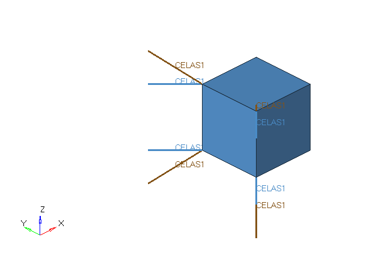
Figure 8. Unit CHEXA Cube Element Model Connected to Springs

Integrate Multiscale Designer Files with OptiStruct

  1. In Multiscale Designer, select the input file (.mic).
  2. Select the Solver Interfaces tab.
  3. In the option for OptiStruct, click the Multiscale Materials tab.
    The Multiscale Designer solver interface for OptiStruct opens.
  4. Make sure that the plugin “dll” and multiscale material data files are pointing to the material subroutine and Multiscale Designer model, respectively.

    Example directory to the material subroutine and Multiscale Designer model are <hwinstallation_directory\hwsolvers\MultiscaleDesigner\win64\plugins\optiStruct\umat.dll> and <working_directory\MultiscaleDesigner\model_name\Mechanical\model_name_mdsMAT.dat>, respectively.

    The number of user-defined variables computed for isotropic damage law is 8, which the terms from damage state variable, equivalent strain, total strain, and Eigen strain.

  5. Change the output folder directory for the plugin data to the model file path, <working_directory\model_name\Mechanical>.

    The generated plugin data file (OptiStruct_plugin_data.fem) contains the LOADLIB I/O and MATUSR cards for running the structural analysis. The LOADLIB I/O Entry is used to implement external subroutines and MATUSR is used to defined user material parameters and properties. These cards are later inserted into OptiStruct input model files (*.fem).

    Note:
    1. The input model file should be in the same folder as the multiscale material. The material subroutines are called into this database through LOADLIB.
    2. The USUBID number in the MATUSR should refer to the multiscale material model ID.

Single-scale Results

Sample cards are generated for Multiscale Designer-OptiStruct integration, with the results of tension and compression test in OptiStruct with the user-defined material.

Elastic properties from homogenization and stress-strain curve from damage law are presented.

Linear Material Characterization

The parameters and values for Failure input properties of cast iron in Nonlinear Material Characterization show that the stress at damage initiation is 126 MPa for tension and 303 MPa for compression. The corresponding time-step, up to which the material is linear is 0.15 s and 0.30 s for tension and compression, respectively. Figure 9 shows the contour plots of x-direction stresses, x-direction strain and y-direction strain from which the elastic properties of the material can be calculated using elasticity equations. In this simulation, the homogenized elastic properties of the material are the same as input properties. This is because the material is assumed to be isotropic.


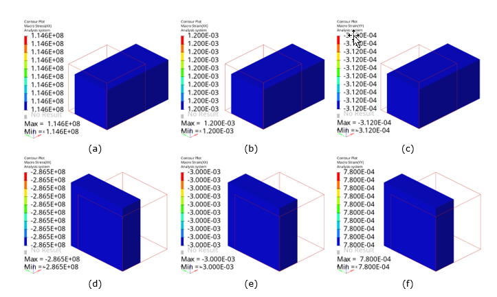
Figure 9. Built-in Macro Simulation in Multiscale Designer (Contour Plots). (a) and (d) x-direction stress in tension and compression, respectively; (b) and (e) x-direction strains in tension and compression, respectively; and (c) and (f) y-direction strains in tension and compression, respectively
The calculated homogenized parameter properties and values are:
Tensile Young’s modulus (GPa), E t MathType@MTEF@5@5@+= feaagKart1ev2aqatCvAUfeBSjuyZL2yd9gzLbvyNv2CaerbuLwBLn hiov2DGi1BTfMBaeXatLxBI9gBaerbd9wDYLwzYbItLDharqqtubsr 4rNCHbGeaGqiVCI8FfYJH8YrFfeuY=Hhbbf9v8qqaqFr0xc9pk0xbb a9q8WqFfeaY=biLkVcLq=JHqpepeea0=as0Fb9pgeaYRXxe9vr0=vr 0=vqpWqaaeaabiGaciaacaqabeaadaqaaqaaaOqaaabaaaaaaaaape Gaamyra8aadaWgaaWcbaWdbiaadshaa8aabeaaaaa@3829@
95.5
Compressive Young’s modulus (GPa), E c MathType@MTEF@5@5@+= feaagKart1ev2aqatCvAUfeBSjuyZL2yd9gzLbvyNv2CaerbuLwBLn hiov2DGi1BTfMBaeXatLxBI9gBaerbd9wDYLwzYbItLDharqqtubsr 4rNCHbGeaGqiVCI8FfYJH8YrFfeuY=Hhbbf9v8qqaqFr0xc9pk0xbb a9q8WqFfeaY=biLkVcLq=JHqpepeea0=as0Fb9pgeaYRXxe9vr0=vr 0=vqpWqaaeaabiGaciaacaqabeaadaqaaqaaaOqaaabaaaaaaaaape Gaamyra8aadaWgaaWcbaWdbiaadshaa8aabeaaaaa@3829@
95.5
Poisson's value, ν MathType@MTEF@5@5@+= feaagKart1ev2aqatCvAUfeBSjuyZL2yd9gzLbvyNv2CaerbuLwBLn hiov2DGi1BTfMBaeXatLxBI9gBaerbd9wDYLwzYbItLDharqqtubsr 4rNCHbGeaGqiVCI8FfYJH8YrFfeuY=Hhbbf9v8qqaqFr0xc9pk0xbb a9q8WqFfeaY=biLkVcLq=JHqpepeea0=as0Fb9pgeaYRXxe9vr0=vr 0=vqpWqaaeaabiGaciaacaqabeaadaqaaqaaaOqaaabaaaaaaaaape GaeqyVd4gaaa@37C4@
0.26

Nonlinear Material Characterization

The stress-strain curve generated from Multiscale Designer is shown in Figure 10. The maximum difference between Multiscale Designer and experiment is 9.6 % at 0.004 strain. At strain values of -0.01 and 0.008, the models are fully damaged; therefore, it is recommended to use the material with a strain value from -0.095 to 0.0076. The stresses corresponding to the fully damaged strains are -0.96 MPa and 184.13 MPa, respectively. The results are plotted against data from experiments 11 and Multiscale Designer.


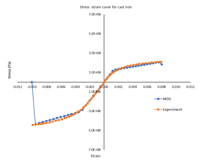
Figure 10. Stress-Strain Curve of Cast Iron from Multiscale Designer and Experiment

Multiscale Designer-OptiStruct Integration

The OptiStruct plugin file generated from Multiscale Designer is illustrated in Figure 11. This file contains information in the LOADLIB I/O and MATUSR cards.


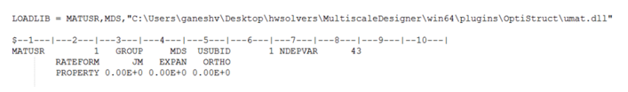
Figure 11. OptiStruct Plugin File from Multiscale Designer

Structural Analysis

NLPARM and NLOUT cards are used for solution control and incremental solution output, respectively, for nonlinear analysis in OptiStruct. In this model, the incremental results are output for each load increment value of 0.05. The material stays linear up to a load factor of 0.175 for tension and 0.2875 for compression. Figure 12 shows the contour plots of x-direction stresses, x-direction strains and y-direction strains for the corresponding load factors. The wireframes in Figure 12 shows the undeformed boundaries.


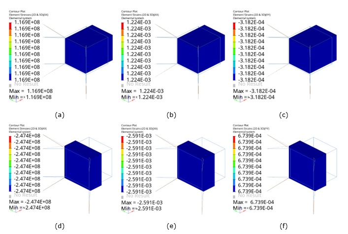
Figure 12. Structural Analysis in OptiStruct (Contour Plots). (a) and (d) x-direction stress in tension and compression, respectively; (b) and (e) x-direction strains in tension and compression, respectively; and (c) and (f) y-direction strains in tension and compression, respectively
Figure 13 depicts the stress-strain curve generated from OptiStruct using MATUSR and LOADLIB. The plot shows that the user-material from Multiscale Designer can be simulated well in OptiStruct.


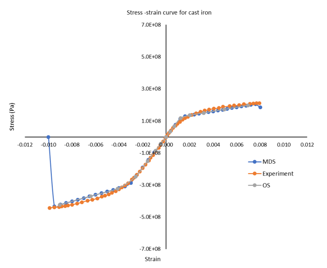
Figure 13. Stress-Strain Curve of Cast Iron

Multiscale Model

The basic steps required to construct a multiscale material model.

Unidirectional fiber-reinforced polymer composite is subjected to tensile load in fiber-axial and fiber-transverse directions. The response of the material is output and validated with experimental data. The first two sections explain the input data required from the Multiscale Designer (MDS). The next two sections explain the procedure to integrate the material in OptiStruct (OS).

Unit Cell Model and Linear Material Characterization

The material model type is selected as multi-scale material characterization. The unit cell is modeled as a fibrous material with a square packing array. The volume fraction of the fiber phase is 65%. Figure 14 represents various unit cell models available in Multiscale Designer for fibrous composites.


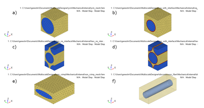
Figure 14. Fibrous Unit Cell Models. (a) square packing array; (b) square packing array with an interface; (c) hexagonal packing array; (d) hexagonal packing array with interface; (e) non-crimp ellipsoidal fabric; and (f) discontinuous fiber packing array

The matrix is modeled with homogeneous elastic properties and the fiber is assumed to be transversely isotropic. Periodic boundary conditions are applied to the unit cell to obtain the homogenized stiffness matrix of the composite.

Linear elastic parameter properties and values of fiber and matrix 13
Young’s modulus of the matrix (GPa), E m MathType@MTEF@5@5@+= feaagKart1ev2aqatCvAUfeBSjuyZL2yd9gzLbvyNv2CaerbuLwBLn hiov2DGi1BTfMBaeXatLxBI9gBaerbd9wDYLwzYbItLDharqqtubsr 4rNCHbGeaGqiVCI8FfYJH8YrFfeuY=Hhbbf9v8qqaqFr0xc9pk0xbb a9q8WqFfeaY=biLkVcLq=JHqpepeea0=as0Fb9pgeaYRXxe9vr0=vr 0=vqpWqaaeaabiGaciaacaqabeaadaqaaqaaaOqaaabaaaaaaaaape Gaamyra8aadaahaaWcbeqaa8qacaWGTbaaaaaa@3814@
3.8
Poisson’s ratio of the matrix, ν m MathType@MTEF@5@5@+= feaagKart1ev2aqatCvAUfeBSjuyZL2yd9gzLbvyNv2CaerbuLwBLn hiov2DGi1BTfMBaeXatLxBI9gBaerbd9wDYLwzYbItLDharqqtubsr 4rNCHbGeaGqiVCI8FfYJH8YrFfeuY=Hhbbf9v8qqaqFr0xc9pk0xbb a9q8WqFfeaY=biLkVcLq=JHqpepeea0=as0Fb9pgeaYRXxe9vr0=vr 0=vqpWqaaeaabiGaciaacaqabeaadaqaaqaaaOqaaabaaaaaaaaape GaeqyVd42damaaCaaaleqabaWdbiaad2gaaaaaaa@3902@
0.32
Longitudinal Young’s modulus of fiber (GPa), E 1 f MathType@MTEF@5@5@+= feaagKart1ev2aqatCvAUfeBSjuyZL2yd9gzLbvyNv2CaerbuLwBLn hiov2DGi1BTfMBaeXatLxBI9gBaerbd9wDYLwzYbItLDharqqtubsr 4rNCHbGeaGqiVCI8FfYJH8YrFfeuY=Hhbbf9v8qqaqFr0xc9pk0xbb a9q8WqFfeaY=biLkVcLq=JHqpepeea0=as0Fb9pgeaYRXxe9vr0=vr 0=vqpWqaaeaabiGaciaacaqabeaadaqaaqaaaOqaaabaaaaaaaaape Gaamyra8aadaqhaaWcbaWdbiaaigdaa8aabaWdbiaadAgaaaaaaa@38E7@
252.25
Transverse Young’s modulus of fiber (GPa), E 2 f MathType@MTEF@5@5@+= feaagKart1ev2aqatCvAUfeBSjuyZL2yd9gzLbvyNv2CaerbuLwBLn hiov2DGi1BTfMBaeXatLxBI9gBaerbd9wDYLwzYbItLDharqqtubsr 4rNCHbGeaGqiVCI8FfYJH8YrFfeuY=Hhbbf9v8qqaqFr0xc9pk0xbb a9q8WqFfeaY=biLkVcLq=JHqpepeea0=as0Fb9pgeaYRXxe9vr0=vr 0=vqpWqaaeaabiGaciaacaqabeaadaqaaqaaaOqaaabaaaaaaaaape Gaamyra8aadaqhaaWcbaWdbiaaigdaa8aabaWdbiaadAgaaaaaaa@38E7@
13.45
Longitudinal Poisson’s ratio, ν 12 MathType@MTEF@5@5@+= feaagKart1ev2aqatCvAUfeBSjuyZL2yd9gzLbvyNv2CaerbuLwBLn hiov2DGi1BTfMBaeXatLxBI9gBaerbd9wDYLwzYbItLDharqqtubsr 4rNCHbGeaGqiVCI8FfYJH8YrFfeuY=Hhbbf9v8qqaqFr0xc9pk0xbb a9q8WqFfeaY=biLkVcLq=JHqpepeea0=as0Fb9pgeaYRXxe9vr0=vr 0=vqpWqaaeaabiGaciaacaqabeaadaqaaqaaaOqaaabaaaaaaaaape GaeqyVd42damaaBaaaleaapeGaaGymaiaaikdaa8aabeaaaaa@3995@
0.02
Transverse Poisson’s ratio, ν 23 MathType@MTEF@5@5@+= feaagKart1ev2aqatCvAUfeBSjuyZL2yd9gzLbvyNv2CaerbuLwBLn hiov2DGi1BTfMBaeXatLxBI9gBaerbd9wDYLwzYbItLDharqqtubsr 4rNCHbGeaGqiVCI8FfYJH8YrFfeuY=Hhbbf9v8qqaqFr0xc9pk0xbb a9q8WqFfeaY=biLkVcLq=JHqpepeea0=as0Fb9pgeaYRXxe9vr0=vr 0=vqpWqaaeaabiGaciaacaqabeaadaqaaqaaaOqaaabaaaaaaaaape GaeqyVd42damaaBaaaleaapeGaaGymaiaaikdaa8aabeaaaaa@3995@
0.3

Nonlinear Material Characterization

The matrix is assumed to obey isotropic damage – bilinear evolution model and the fiber is assumed to follow orthotropic damage – bilinear evolution, for simulating the nonlinear behavior of the material.

The nonlinear input parameter properties and values for damage law 13 are:
Stress at damage initiation (MPa), σ 0 m MathType@MTEF@5@5@+= feaagKart1ev2aqatCvAUfeBSjuyZL2yd9gzLbvyNv2CaerbuLwBLn hiov2DGi1BTfMBaeXatLxBI9gBaerbd9wDYLwzYbItLDharqqtubsr 4rNCHbGeaGqiVCI8FfYJH8YrFfeuY=Hhbbf9v8qqaqFr0xc9pk0xbb a9q8WqFfeaY=biLkVcLq=JHqpepeea0=as0Fb9pgeaYRXxe9vr0=vr 0=vqpWqaaeaabiGaciaacaqabeaadaqaaqaaaOqaaabaaaaaaaaape Gaeq4Wdm3damaaCaaaleqabaWdbiaaicdacaWGTbaaaaaa@39C7@
126.0
Strain at ultimate stress, ε 1 m MathType@MTEF@5@5@+= feaagKart1ev2aqatCvAUfeBSjuyZL2yd9gzLbvyNv2CaerbuLwBLn hiov2DGi1BTfMBaeXatLxBI9gBaerbd9wDYLwzYbItLDharqqtubsr 4rNCHbGeaGqiVCI8FfYJH8YrFfeuY=Hhbbf9v8qqaqFr0xc9pk0xbb a9q8WqFfeaY=biLkVcLq=JHqpepeea0=as0Fb9pgeaYRXxe9vr0=vr 0=vqpWqaaeaabiGaciaacaqabeaadaqaaqaaaOqaaabaaaaaaaaape GaeqyTdu2damaaCaaaleqabaWdbiaaigdacaWGTbaaaaaa@39AC@
0.1
Damage input properties of the fiber
Stress at damage initiation – longitudinal direction (GPa), σ 1 0 f MathType@MTEF@5@5@+= feaagKart1ev2aqatCvAUfeBSjuyZL2yd9gzLbvyNv2CaerbuLwBLn hiov2DGi1BTfMBaeXatLxBI9gBaerbd9wDYLwzYbItLDharqqtubsr 4rNCHbGeaGqiVCI8FfYJH8YrFfeuY=Hhbbf9v8qqaqFr0xc9pk0xbb a9q8WqFfeaY=biLkVcLq=JHqpepeea0=as0Fb9pgeaYRXxe9vr0=vr 0=vqpWqaaeaabiGaciaacaqabeaadaqaaqaaaOqaaabaaaaaaaaape Gaeq4Wdm3damaaDaaaleaapeGaaGymaaWdaeaapeGaaGimaiaadAga aaaaaa@3A9A@
4.2
Strain at ultimate stress – longitudinal direction, ε 1 1 f MathType@MTEF@5@5@+= feaagKart1ev2aqatCvAUfeBSjuyZL2yd9gzLbvyNv2CaerbuLwBLn hiov2DGi1BTfMBaeXatLxBI9gBaerbd9wDYLwzYbItLDharqqtubsr 4rNCHbGeaGqiVCI8FfYJH8YrFfeuY=Hhbbf9v8qqaqFr0xc9pk0xbb a9q8WqFfeaY=biLkVcLq=JHqpepeea0=as0Fb9pgeaYRXxe9vr0=vr 0=vqpWqaaeaabiGaciaacaqabeaadaqaaqaaaOqaaabaaaaaaaaape GaeqyTdu2damaaDaaaleaapeGaaGymaaWdaeaapeGaaGymaiaadAga aaaaaa@3A7F@
0.017
Stress at damage initiation – transverse direction (MPa), σ 2 0 f MathType@MTEF@5@5@+= feaagKart1ev2aqatCvAUfeBSjuyZL2yd9gzLbvyNv2CaerbuLwBLn hiov2DGi1BTfMBaeXatLxBI9gBaerbd9wDYLwzYbItLDharqqtubsr 4rNCHbGeaGqiVCI8FfYJH8YrFfeuY=Hhbbf9v8qqaqFr0xc9pk0xbb a9q8WqFfeaY=biLkVcLq=JHqpepeea0=as0Fb9pgeaYRXxe9vr0=vr 0=vqpWqaaeaabiGaciaacaqabeaadaqaaqaaaOqaaabaaaaaaaaape Gaeq4Wdm3damaaDaaaleaapeGaaGymaaWdaeaapeGaaGimaiaadAga aaaaaa@3A9A@
75.0
Strain at ultimate stress – transverse direction, ε 2 1 f MathType@MTEF@5@5@+= feaagKart1ev2aqatCvAUfeBSjuyZL2yd9gzLbvyNv2CaerbuLwBLn hiov2DGi1BTfMBaeXatLxBI9gBaerbd9wDYLwzYbItLDharqqtubsr 4rNCHbGeaGqiVCI8FfYJH8YrFfeuY=Hhbbf9v8qqaqFr0xc9pk0xbb a9q8WqFfeaY=biLkVcLq=JHqpepeea0=as0Fb9pgeaYRXxe9vr0=vr 0=vqpWqaaeaabiGaciaacaqabeaadaqaaqaaaOqaaabaaaaaaaaape GaeqyTdu2damaaDaaaleaapeGaaGymaaWdaeaapeGaaGymaiaadAga aaaaaa@3A7F@
0.05

For nonlinear material characterization in fiber-axial and fiber-transverse direction, two laminate layups with unit thickness are created with orientations 0° and 90°, respectively. Each laminate is subjected to Unnotched Tensile/Compression macro simulation with different loading rates.

The input values for the macro simulations are:
Loading rate – Fiber axial direction test (/s)
0.05
Maximum strain - Fiber axial direction test
0.05
Loading rate – Fiber transverse direction test (/s)
0.017
Maximum strain - Fiber transverse direction test
0.017

The output data files are generated in the material model directory and the stress-strain curve data will export to an Excel spreadsheet file in <material_model_directory\model_name\mechanical\model_name_NLmatl.xlsx>.

Integrate Multiscale Designer Files with Multiscale Designer-OptiStruct

  1. In Multiscale Designer solver interface for OptiStruct, click the Homogenized Materials tab.
  2. Set the card images to MAT2, MAT8, MAT9 or MAT9ORT.
  3. Click the Multiscale Materials tab and set the output file path for the OptiStruct plugin “dll”.
  4. In the multiscale material data file, browse the file path to <material_model_directory\model_name\mechanical\model_name_mdsMAT.dat>.

    The number of user-defined variables computed for orthotropic damage law is 8, which involves the terms from the damage state variable, equivalent strain, total strain, and eigen strain.

  5. By default, the OptiStruct plugin data files are output to <material_model_directory\Macro\Mechanical\optiStruct_plugin_data.fem>.

Multiscale Results

Sample cards are generated for Multiscale Designer-OptiStruct integration with OptiStruct test results.

Elastic properties from homogenization and stress-strain curve from damage law are presented.

Unit Cell Model and Linear Material Characterization

Figure 15 represents the square fiber packing array generated from Multiscale Designer. The relative radius of the fiber with respect to the unit cell size for the fiber volume fraction is 0.45.


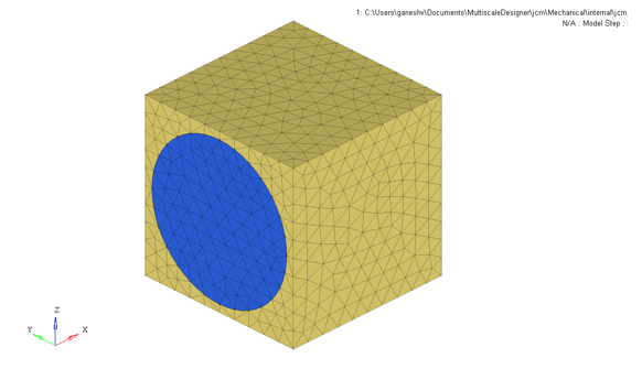
Figure 15. Unit Cell Model of Square Packing Array . with Fiber Volume Fraction = 65%
Homogenized elastic properties of the fiber/matrix composite. Nonlinear material characterization. All these values are available in an Excel spreadsheet in <material_model_directory\model_name\mechanical\model_name_Lmatl.xlsx>.
Longitudinal Young’s modulus (GPa), E 1 c MathType@MTEF@5@5@+= feaagKart1ev2aqatCvAUfeBSjuyZL2yd9gzLbvyNv2CaerbuLwBLn hiov2DGi1BTfMBaeXatLxBI9gBaerbd9wDYLwzYbItLDharqqtubsr 4rNCHbGeaGqiVCI8FfYJH8YrFfeuY=Hhbbf9v8qqaqFr0xc9pk0xbb a9q8WqFfeaY=biLkVcLq=JHqpepeea0=as0Fb9pgeaYRXxe9vr0=vr 0=vqpWqaaeaabiGaciaacaqabeaadaqaaqaaaOqaaabaaaaaaaaape Gaamyra8aadaqhaaWcbaWdbiaaigdaa8aabaWdbiaadogaaaaaaa@38E4@
165.4
Transverse Young’s modulus (GPa), E 1 t MathType@MTEF@5@5@+= feaagKart1ev2aqatCvAUfeBSjuyZL2yd9gzLbvyNv2CaerbuLwBLn hiov2DGi1BTfMBaeXatLxBI9gBaerbd9wDYLwzYbItLDharqqtubsr 4rNCHbGeaGqiVCI8FfYJH8YrFfeuY=Hhbbf9v8qqaqFr0xc9pk0xbb a9q8WqFfeaY=biLkVcLq=JHqpepeea0=as0Fb9pgeaYRXxe9vr0=vr 0=vqpWqaaeaabiGaciaacaqabeaadaqaaqaaaOqaaabaaaaaaaaape Gaamyra8aadaqhaaWcbaWdbiaaigdaa8aabaWdbiaadogaaaaaaa@38E4@
8.8
Longitudinal Poisson’s ratio, ν 12 c MathType@MTEF@5@5@+= feaagKart1ev2aqatCvAUfeBSjuyZL2yd9gzLbvyNv2CaerbuLwBLn hiov2DGi1BTfMBaeXatLxBI9gBaerbd9wDYLwzYbItLDharqqtubsr 4rNCHbGeaGqiVCI8FfYJH8YrFfeuY=Hhbbf9v8qqaqFr0xc9pk0xbb a9q8WqFfeaY=biLkVcLq=JHqpepeea0=as0Fb9pgeaYRXxe9vr0=vr 0=vqpWqaaeaabiGaciaacaqabeaadaqaaqaaaOqaaabaaaaaaaaape GaeqyVd42damaaDaaaleaapeGaaGymaiaaikdaa8aabaWdbiaadoga aaaaaa@3A8E@
0.11
Transverse Poisson’s ratio, ν 23 c MathType@MTEF@5@5@+= feaagKart1ev2aqatCvAUfeBSjuyZL2yd9gzLbvyNv2CaerbuLwBLn hiov2DGi1BTfMBaeXatLxBI9gBaerbd9wDYLwzYbItLDharqqtubsr 4rNCHbGeaGqiVCI8FfYJH8YrFfeuY=Hhbbf9v8qqaqFr0xc9pk0xbb a9q8WqFfeaY=biLkVcLq=JHqpepeea0=as0Fb9pgeaYRXxe9vr0=vr 0=vqpWqaaeaabiGaciaacaqabeaadaqaaqaaaOqaaabaaaaaaaaape GaeqyVd42damaaDaaaleaapeGaaGymaiaaikdaa8aabaWdbiaadoga aaaaaa@3A8E@
0.34

Nonlinear Material Characterization

Figure 16 and Figure 17 show the stress-strain curve generated from Multiscale Designer for fiber-axial and fiber-transverse direction tensile tests. These values are plotted over experimental data. 13 The maximum difference in tensile yield strength between Multiscale Designer and experiment is 6.0 % for the fiber-axial direction test and 11.3 % for the fiber-transverse direction test.


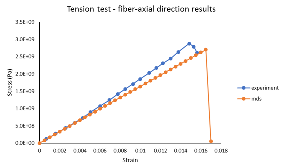
Figure 16. Comparison of Stress-Strain Curves. fiber-axial tensile test from Multiscale Designer and experiment


Figure 17. Stress-Strain Curve. fiber-transverse tensile test from Multiscale Designer and experiment

Multiscale Designer-OptiStruct Integration

A MAT9ORT material file generated from Multiscale Designer is illustrated in Figure 18. These files are to be used in OptiStruct to run any structural analysis. The OptiStruct plugin file which contains the LOADLIB I/O and MATUSR cards is the same as in Figure 11.


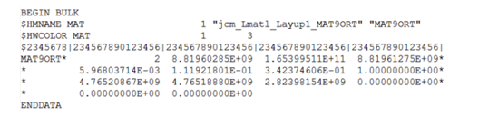
Figure 18. Homogenized Composite Properties in OptiStruct MAT9ORT Format
1 Chaboche, J. L., K. Dang Van, and G. Cordier. "Modelization of the strain memory effect on the cyclic hardening of 316 stainless steel." (1979).
2 Chaboche, Jean-Louis, and G. Rousselier. "On the plastic and viscoplastic constitutive equations—Part II: application of internal variable concepts to the 316 stainless steel." (1983): 159-164.
3 Chaboche, Jean-Louis. "Time-independent constitutive theories for cyclic plasticity." International Journal of plasticity 2.2 (1986): 149-188.
4 Chaboche, Jean-Louis. "Constitutive equations for cyclic plasticity and cyclic viscoplasticity." International journal of plasticity 5.3 (1989): 247-302.
5 Chaboche, J. L., and D. Nouailhas. "Constitutive modeling of ratchetting effects—part i: experimental facts and properties of the classical models." (1989): 384-392.
6 Chaboche, Jean-Louis. "On some modifications of kinematic hardening to improve the description of ratchetting effects." International journal of plasticity 7.7 (1991): 661-678.
7 Lemaitre, Jean, and Jean-Louis Chaboche. Mechanics of solid materials. Cambridge university press, 1994.
8 Broggiato, Giovanni B., Francesca Campana, and Luca Cortese. "The Chaboche nonlinear kinematic hardening model: calibration methodology and validation." Meccanica 43.2 (2008): 115-124.
9 Chaboche, Jean-Louis. "A review of some plasticity and viscoplasticity constitutive theories." International journal of plasticity 24.10 (2008): 1642-1693
10 Altair Engineering Inc. 2018. Multiscale Designer: User Manual. Troy, MI
11 Downing, S.D., 1984. “Modeling Cyclic Deformation and Fatigue Behavior of Cast Iron under Uniaxial Loading,” Report No. 11, University of Illinois at Urbana-Champaign, IL
12 Fish, J., 2014. Practical Multiscaling. John Wiley & Sons, Ltd.
13 Yuan, Z., Crouch, R., Wollschlager, J., Shojaei, A., Fish, J., 2016. “Assessment of Altair Multiscale Designer for damage tolerant design principles (DTDP) of advanced composite aircraft structures,” Journal of Composite Materials, 51(10): 1379-1391