Multibody Dynamics Simulation
A multibody system is defined to be an assembly of sub-systems (bodies, components, or sub-structures).
The motion of the sub-systems may be kinematically constrained and each sub-system or component may undergo large translational and rotational displacements.
Bodies can be considered rigid or flexible. Rigid bodies do not undergo deformations. Rigid body motion can be described completely by using six generalized coordinates. The resulting mathematical model is highly nonlinear. Neglecting the body deformations can lead to inaccurate results. Therefore, some of the bodies are considered flexible, that is they can undergo deformations. Modal reduction procedures are used to include flexible bodies in multibody dynamics simulations.
Joints, force elements, and controls connect the bodies. Initial velocities, forces, and motions may be applied to the system.

Figure 1. Multibody System
This implementation is targeted at the typical finite-element user who wants to solve multibody dynamics problems in the context of a finite element model, and is still somewhat limited. HyperMesh is used for modeling. All geometry entities are defined in terms of a finite element mesh. Flexible body modeling is fully integrated.
HyperStudy can be used for optimization. Shape optimization of rigid and flexible bodies is available through the use of HyperMorph.
Transient Analysis
Transient Analysis is used to calculate the response of a multibody system to time-dependent loads and motions.
Forces and motions are time-dependent. Body initial conditions define the initial body velocities, while joint initial conditions define the initial displacement of a particular joint.
The results of a transient analysis are displacements, velocities, accelerations, forces, as well as modal contributions to stresses and strains in flexible bodies. The responses are usually time-dependent.
The matrix is the mass matrix, the vector is the vector of external forces, and the vector represents the generalized coordinates. Stiffness, damping, constraint forces, external loads, and gravity are all included in the external force vector . An initial and maximum integration time step, an end time, and integrator tolerance need to be defined.
Two analyses, kinematic and dynamic, are defined depending on the degree of freedom of the system analysis.
A kinematic simulation is performed if all degrees of freedom are constrained through appropriate joints and/or motions, making it a zero degree of freedom model. A kinematics simulation finds a system configuration that satisfies all kinematic constraints and motion equations at any given time. The configuration is obtained by solving a system of nonlinear algebraic equations representing constraints.
During a kinematic simulation, there is no need to integrate the differential equations of motion because the system configuration is fully determined by solving the constraint and motion equations alone. Even though forces are not used to compute the kinematics solution, joint reaction forces can be computed at any given time. The mass and inertia properties of bodies involved, and external forces acting on them, do not affect the resultant system configuration, but they do affect the joint reaction forces requested as outputs.
A dynamic simulation is employed whenever the model has one or more degrees of freedom. A dynamic simulation involves integrating the differential equations of motion subject to nonlinear algebraic equations representing kinematics constraints. In other words, the solution is obtained by solving a mixed system of differential-algebraic equations.
The resultant solution takes into account various dynamic effects and is dependent upon mass and inertia properties of bodies, damping within the system, and applied forces and motions. Additional simulation parameters, such as the integration scheme, integration time step, convergence tolerance, etc. could also affect the solution and; therefore, need to be specified appropriately.
If a simulation type of transient is requested, the solver automatically determines whether to run a kinematic or dynamic solution from the degree of freedom.
- VSTIFF (Default) - Implicit integrator that utilizes the Variable Coefficient Differential Equation Solver (VODE). It is suited for stiff and non-stiff problems.
- MSTIFF - Implicit integrator that utilizes the Modified Extended Backward Differentiation Formula (MEBDF) to solve the nonlinear equations of motion. It is suited for stiff problems.
- ABAM (Adams-Bashforth-Adams-Moulton) - Explicit integrator that uses a finite differences scheme to solve the nonlinear equations of motion. This integrator is suitable for systems that are non-stiff.
A multibody subcase needs to be defined in the input deck. Only one such subcase can be used in a model. The simulation type "static" is defined on an MBSIM Bulk Data Entry which must be referenced through a subcase statement MBSIM. The MBSIM Bulk Data Entry also defines the integrator, end time, and time step. A sequence of several simulations of different types can be defined by referring to an MBSEQ Bulk Data statement instead. Loads and motions are referenced on MLOAD and MOTION Subcase Information Entries, respectively. Initial velocities do not apply here. SPC type constraints in Multibody Dynamics analysis are allowed only for MBD-ESL optimization of a flexible body if displacements are used as constraints. Further information on loads and boundary conditions can be obtained from Applied Forces and Motions and Initial Velocity.
The unit system for the simulation can be defined using a DTI, UNITS Bulk Data Entry.
Static Analysis
A static simulation is also called an equilibrium simulation. The system must have at least one degree of freedom to undergo a static simulation and an initial configuration must be specified.
A zero degree of freedom system is always considered to be in static equilibrium once all of the kinematic constraints are satisfied.
Starting with the user-specified initial configuration, a final configuration is arrived at iteration-by-iteration, such that there are no unbalanced forces or torques on any of the bodies in the system and all of the kinematics constraints are satisfied. All of the velocities and accelerations are set to zero.
A multibody subcase needs to be defined in the input deck. Only one such subcase can be used in a model. The simulation type "static" is defined on an MBSIM Bulk Data Entry which must be referenced through a subcase statement MBSIM. The MBSIM Bulk Data Entry also defines the integrator, end time, and time step. A sequence of several simulations of different types can be defined by referring to an MBSEQ Bulk Data statement instead. Loads and motions are referenced on MLOAD and MOTION Subcase Information Entries, respectively. Initial velocities do not apply here. SPC type constraints in Multibody Dynamics analysis are allowed only for MBD-ESL optimization of a flexible body if displacements are used as constraints. Further information on loads and boundary conditions can be obtained from Applied Forces and Motions and Initial Velocity.
The unit system for the simulation can be defined using a DTI, UNITS Bulk Data Entry.
Quasi-static Analysis
A quasi-static simulation is a sequence of static simulation steps applied to a model over a given duration at specified intervals.
A quasi-static simulation is employed when you have time-dependent forces or motions in the model and you want a static equilibrium configuration at every time step. The system must have at least one degree of freedom to undergo a quasi-static simulation and you must specify the initial configuration.
For the first time step, the user-specified initial configuration is used as a starting point, whereas for all other time-steps, a configuration from the previous time step is used as the starting point for equilibrium simulation at that time step. A final configuration is arrived at iteration-by-iteration, such that there are no unbalanced forces or torques on any of the bodies in the system and all of the kinematic constraints are satisfied at that time step. For every step, all velocities and accelerations are set to zero.
A multibody subcase needs to be defined in the input deck. Only one such subcase can be used in a model. The simulation type "static" is defined on an MBSIM Bulk Data Entry which must be referenced through a subcase statement MBSIM. The MBSIM Bulk Data Entry also defines the integrator, end time, and time step. A sequence of several simulations of different types can be defined by referring to an MBSEQ Bulk Data statement instead. Loads and motions are referenced on MLOAD and MOTION Subcase Information Entries, respectively. Initial velocities do not apply here. SPC type constraints in Multibody Dynamics analysis are allowed only for MBD-ESL optimization of a flexible body if displacements are used as constraints. Further information on loads and boundary conditions can be obtained from Applied Forces and Motions and Initial Velocity.
The unit system for the simulation can be defined using a DTI, UNITS Bulk Data Entry.
Linear Analysis
In Linearization Analysis, the nonlinear representations of force, motion, stiffness, or damping are linearized.
A linearization can be performed on these models to prepare a model for use with Matlab or to obtain eigenmodes characteristics of the model. In the case of performing a linear analysis on the mechanical system, optional files of type eig_info, Simulink MDL, and Matlab ABCD matrices are available to be exported.
A multibody subcase needs to be defined in the input deck. Only one such subcase can be used in a model. The simulation type "static" is defined on an MBSIM Bulk Data Entry which must be referenced through a subcase statement MBSIM. The MBSIM Bulk Data Entry also defines the integrator, end time, and time step. A sequence of several simulations of different types can be defined by referring to an MBSEQ Bulk Data statement instead. Loads and motions are referenced on MLOAD and MOTION Subcase Information Entries, respectively. Initial velocities do not apply here. SPC type constraints in Multibody Dynamics analysis are allowed only for MBD-ESL optimization of a flexible body if displacements are used as constraints. Further information on loads and boundary conditions can be obtained from Applied Forces and Motions and Initial Velocity.
The unit system for the simulation can be defined using a DTI, UNITS Bulk Data Entry.
Bodies
Bodies are the model elements that have mass and inertia. Bodies can be rigid or flexible.
A rigid body has only mass and inertia, and does not deform during the simulation. An initial velocity can be assigned. Mass and inertia information can be omitted for kinematic, static, and quasi-static simulations. It does not affect displacement, velocity, and acceleration results of kinematic simulation or displacement results of a static or a quasi-static simulation. Mass and inertia information must be correctly specified if joint-reaction forces are of interest in kinematic, static, or quasi-static simulations.
Where, are the modal coordinates which are to be determined by the multibody dynamics analysis. The set of orthogonal modes is determined in a Component Mode Synthesis (CMS). Depending on the model, CMS can be performed as a pre-processing step using a special simulation (Finite Element Analysis (Superelements)). Besides displacements, velocities, and accelerations, stresses and strains can also be computed for flexible bodies.
One special rigid body is the ground body. It describes the reference environment, and does not add any degrees of freedom to the system. It is at absolute rest. Any grounded body is merged into one.
Bodies are defined in terms of a finite element model. A body is formed by a group of properties, elastic, rigid, and mass elements as well as grid points.
Rigid bodies are defined on a PRBODY entry. Mass and inertia are either determined from the geometric entities or can be entered on PRBODY.
The ground body is defined using the GROUND Bulk Data Entry.
Flexible bodies are defined using the PRBODY Bulk Data Entry. The interface grid points are automatically determined or are defined on PRBODY using the FLXNODE flag. The procedure, as described in Direct Matrix Approach, is applied to each PRBODY definition. The procedure is fully integrated in the multibody dynamics solution sequence, where flexh3d files are generated for multiple flexible bodies in the same model. The parameter PARAM, FLEXH3D may be used to control the regeneration of flexh3d files for subsequent runs.
Markers
A marker is a coordinate system attached to a body at a geometric point. Markers are used as a reference for joints, compliant elements, applied loads, and output requests.
Markers are defined using a grid point and a coordinate system. The MARKER Bulk Data Entry is used.
Constraints
Typical types of constraints like joints, couplers, and high-pair joints can be defined. Higher-pair joints include point-to-curve, point-to-surface, and curve-to-curve constraints. They can connect rigid bodies, flexible bodies, or a rigid and flexbody.
The multibody system must be sufficiently constrained.
Before running the solver, any redundant constraints in the model are removed. Since the constraint forces associated with redundant constraints are set to zero, it is important to review all of the constraints in the model to make sure they are physically meaningful and that there are no unintended redundant constraints.
| Joint Type | Constrained Degrees of Freedom | Number of GRIDs | |
|---|---|---|---|
| Translation | Rotation | ||
| Fixed | 3 | 3 | 2 |
| Revolute | 3 | 2 | 3 |
| Translational | 2 | 3 | 3 |
| Cylindrical | 2 | 2 | 3 |
| Universal (development source only) | 3 | 1 | 4 |
| Planar | 1 | 2 | 3 |
| Ball | 3 | 0 | 2 |
| Perpendicular | 0 | 1 | 4 |
| Parallel axes | 0 | 2 | 4 |
| Orientation | 0 | 3 | 2 |
| In-plane | 1 | 0 | 4 |
| Inline | 2 | 0 | 3 |
| Constant velocity | 3 | 1 | 4 |
Couplers are constraints between the translational and/or the rotational motion of two or three joints. They are defined using the COUPLER Bulk Data Entry.
- Higher-pair Joint Type
- Bulk Data Entry
- Point-to-curve
- MBPTCV
- Point-to-deformable curve
- MBPTDCV
- Point-to-deformable surface
- MBPTDSF
- Curve-to-curve
- MBCVCV
These entries refer to the parametric curve definition (MBPCRV), deformable curve definition (MBPTDCV), and deformable surface definition (MBDSRF).
Contact
The contact modeling capability for multibody dynamics can handle complex contact scenarios between rigid bodies and rigid and flexible bodies.
For the definition you have to identify geometries on one body that can contact a different set of geometries on a second body. You also specify the contact material properties such as coefficient of restitution and friction. The solver monitors the proximity of the specified geometries to each other. When contact between the two sets of geometry occurs, a force based on the defined physical properties is generated. This represents the contact force. Both normal and frictional forces are modeled. When the bodies separate, the force becomes zero.
- Modeling the geometry of the bodies that are in contact
- Detecting the onset of contact
- Applying the contact force
- Detecting the end of a contact "incident" and removing the contact force
Two contact types are available: Rigid body to rigid body (MBCNTR) which is defined as the contact of two element sets (SET) and rigid to flexible body (MBCNTDS) which is defined as the contact between a node set (SET) and a deformable surface. The deformable surface must be defined by the MBDSRF Bulk Data Entry.
- The point of contact and surface normal vector
- The magnitude and direction of the normal and friction forces
Once the point of contact and surface normal vector are known, the normal and friction force magnitudes are computed using a penalty-based Poisson contact normal force model. The two primary inputs to this model are the penalty and the coefficient of restitution (COR). COR is defined as the ratio of relative speed of separation to the relative speed of approach of the colliding bodies. A COR of 1.0 implies a perfectly elastic collision and a COR of 0.0 represents a perfectly plastic collision. One may think of the COR as damping and penalty as stiffness. Too high of a penalty value may cause numerical difficulties, while too small of a value may lead to excessive penetration. Some fine-tuning of these two parameters is usually required to reach stable and accurate results.
- Current slip speed at the point of contact
- Coefficient of static friction
- Coefficient of dynamic friction
- Friction transition slip speed at which the full value of is used for the coefficient of friction.
- Dynamic friction slip speed at which the full value of is used for the coefficient of friction.
- Friction force that is to be applied. The friction force opposes the direction of the slip velocity.
Compliant Elements
Compliant Elements are bushings, spring-dampers, and beams.
For each, the relevant information such as stiffness, damping, preload, attachment markers, etc. needs to be defined. Stiffness and damping value numbers should correctly represent the actual system and must be physically meaningful. Otherwise, the system may inadvertently turn out to be numerically stiff, even though the physical system may not be.
Compliant elements can be defined with respect to grid points or with respect to markers.
CMBEAM and CMBEAMM Bulk Data Entries define beam elements.
CMBUSH and CMBUSHM Bulk Data Entries define bushing elements. A bushing element has linear stiffness and damping properties.
CMSPDP and CMSPDPM Bulk Data Entries define spring-damper elements.
Applied Forces and Motions
Forces and moments can be present in the system. There are action-only forces which are applied to one point, and action-reaction forces which are applied to two points.
Force components can be a constant value, a curve, an expression, or a user-written subroutine.
A special force is gravity. Acceleration is applied to a body and from mass and acceleration, the gravitational force is computed.
Motion is a scalar constraint to the system. Displacement, velocity, and acceleration-type motions are possible. The motion must depend only on time and not on any other measures in the model that could change during the simulation. In other words, at every time step with only time as the independent parameter, the solver should be able to evaluate the expression completely without using any other information about the model. For example, the motion cannot depend upon displacement or velocity or acceleration between two points in the model.
Motion can be specified as a constant value, a curve, an expression, or user-written subroutine. Motion is either defined as motion between two points or joint motion. When a motion is applied on a joint, one joint degree of freedom is controlled as a function of time. When a motion is applied between two points, movement along a user-specified direction is controlled as a function of time.
Forces are always defined at grid points, and can be applied to one grid point (action-only) or two (action-reaction). The MBFRC Bulk Data Entry defines constant force; the MBFRCC Bulk Data Entry defines force by a curve; and the MBFRCE Bulk Data Entry defines a force by equation.
Moments are always defined at grid points, and can be applied to one grid point (action-only) or two (action-reaction). The MBMNT Bulk Data Entry defines constant moment; the MBMNTC Bulk Data Entry defines moment by a curve; and the MBMNTE Bulk Data Entry defines a moment by equation.
GRAV defines the gravity acceleration.
The MLOAD Bulk Data Entry can be used to derive force and moment set combinations.
Motion can be defined as grid point motion or as joint motion. Grid point motion can be applied to one grid point or two (relative motion). The MOTNG Bulk Data Entry defines constant motion; the MOTNGC Bulk Data Entry defines motion by a curve, and MOTNGE Bulk Data Entry defines motion by an equation. Joint motion can be applied to translational or revolute joints only. The MOTNJ Bulk Data Entry defines constant motion; the MOTNJC Bulk Data Entry defines motion by a curve, and MOTNJE Bulk Data Entry defines motion by an equation. The MOTION Bulk Data Entry can be used to derive motion set combinations.
Initial Velocity
Initial velocity is part of the problem formulation of the equation of motion. It can be applied to bodies or to cylindrical, translational, and rotational joints.
The INVELB Bulk Data Entry defines body initial velocity. The entry INVEL can be used to derive initial velocity set combinations.
Function Expressions
Function Expressions formulate relationships as functions of time, displacements, velocities, acceleration, forces, etc.
Expressions can be used in many places. If geometric points are used in an equation, they are always related to markers.
The MBVAR Bulk Data Entry is used to define equations.
Results
The primary results in a multibody dynamics analysis are the motions of the bodies.
They are written as nodal displacements, velocities, and accelerations. For flexible bodies, element results such as deformations, stresses, and strains are derived from those results. These results can be displayed in an animation of the entire system in a graphical toll such as HyperView. Aside from the full nodal results, the solver provides a more compressed form of animation data only for multibody dynamics analysis that can only be displayed in HyperView, where HyperView does many of the typical transformations and final computations.
See Results of a Finite Element Analysis to find more information on how to post-process nodal and elemental results.
Measures like body displacements, velocities, accelerations, joint forces, and user-defined expressions are being written as time history. Marker time history can be written upon request. These results can be plotted in a graphical plotting tool such as HyperGraph.
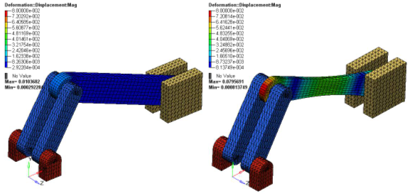
Figure 2.