OS-T: 1570 Nonlinear Transient Analysis of Crank Slider
In this tutorial, an existing finite element model of a slider crank is used to demonstrate how to perform Nonlinear Transient Analysis using OptiStruct.
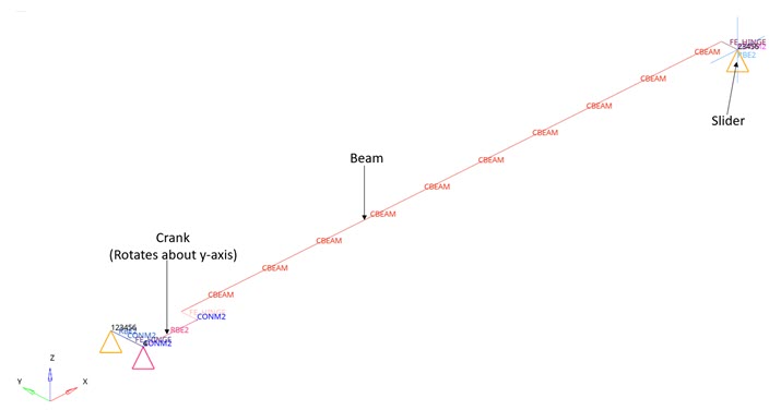
Figure 1. Model and loading description
Figure 1 illustrates the structural model used for this tutorial: A slider crank is a four-link mechanism with three revolute joints and one sliding joint. The mechanism is completely constrained at one end and transient load are applied to the crank. The Nonlinear transient analysis is run for a total time of 1 second with the time being divided into 200 increments (that is step time equal to 0.005). A concentrated mass is defined at the center of the slider, both the ends of the crank and at the hinge.
You will be simulating the Slider Crank model, which is modeled using beam/solid elements. The crank will be rotated by 180 degrees about the z-axis by applying appropriate constraints on other links.
- One with beam elements
- One with solid elements
Launch HyperMesh and Set the OptiStruct User Profile
Import the Model
Set Up the Model
Create the Material
Here you will define the beam material.
Create the Property
Here you will create the beam property.
Apply Loads and Boundary Conditions
Create TABLED1 Curve
-
In the Model Browser, right-click on the
TABLED1 curve and select Edit
enter the values:
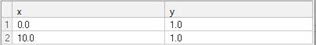
Figure 2.
Create TSTEP Load Collector
Here you will define the hyper elastic behavior of the implant.
- In the Model Browser, right-click and select .
- For Name, enter tstep.
- Click Color and select a color from the color palette.
- For Card Image, select TSTEP from the drop-down menu.
- For TSTEP_NUM, enter 1 and press Enter.
- For N, enter the number of time steps as 200.
- For DT, enter the time increment of 0.005.
- Click Close.
Create SPC Load Collector
-
Click create.
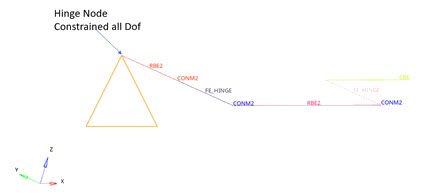
Figure 3. Constraints on the hinge node -
Select the center node of the slider (Figure 4) and check all DoFs; except DoF1.
This indicates that DoF1 is the only active Degree of Freedom.
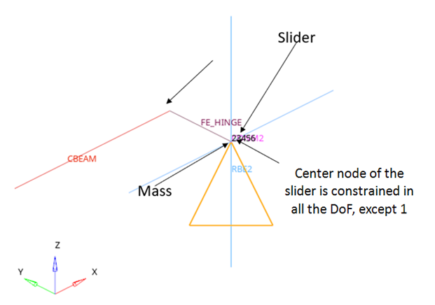
Figure 4. Constraints applied to the center node of the slider
Create SPC1 Load Collector
One more SPC load collector is created here.
-
Check all Degrees of Freedom (DoFs); except DoF4.
This indicates that DoF4 is the only active Degree of Freedom.
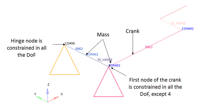
Figure 5. Constraints applied to the first node of the crank
Create SPCD Load Collector
Create SPCADD Load Collector
-
Click on the Table icon
 next to the Data
field and enter the following values in the pop-out window as:
next to the Data
field and enter the following values in the pop-out window as:
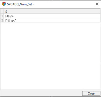
Figure 6.
Create GRAV Load Collector
- In the Model Browser, right-click and select .
- For Name, enter grav.
- Click Color and select a color from the color palette.
- For Card Image, select GRAV from the drop-down menu.
- For G, enter 9.8.
- For N3, enter -1.0.
Create a TLOAD Load Collector
- In the Model Browser, right-click and select .
- For Name, enter tload.
- Click Color and select a color from the color palette.
- For Card Image, select TLOAD1 from the drop-down menu.
- For EXCITEID , click .
- In the Select Loadcol dialog, select spcd from the list of load collectors.
- For Type, select VELO.
- For TID, select table.
Create tload_grav Load Collector
Here you will create one more TLOAD load collector.
- In the Model Browser, right-click and select .
- For Name, enter tload_grav.
- Click Color and select a color from the color palette.
- For Card Image, select TLOAD from the drop-down menu.
- For EXCITED, click .
- In the Select Loadcol dialog, select grav from the list of load collectors.
- For TYPE, select LOAD.
- For TID, select table.
Create a DLOAD Load Collector
- In the Model Browser, right-click and select .
- For Name, enter dload.
- Click Color and select a color from the color palette.
- For Card Image, select DLOAD from the drop-down list.
- For S (scale factor), enter 1.0.
- For DLOAD_NUM, enter 2.
- For data, select tload and tload_grav and enter 1 as the scale factor for both loads.
- Click Close.
Create NLPARM Load Collector
The nonlinear implicit parameters are defined.
- In the Model Browser, right-click and select .
- For Name, enter nlParm.
- Click Color and select a color from the color palette.
- For Card Image, select NLPARM from the drop-down menu.
- For NINC, enter 200.
- For DT, enter 0.005.
Create NLADAPT Load Collector
- In the Model Browser, right-click and select .
- For Name, enter nladapt.
- Click Color and select a color from the color palette.
- For Card Image, select NLADAPT from the drop-down menu.
- For DTMAX, enter 0.005.
- For DTMIN, enter 1e-05.
- For NCUTS, enter 5.
Create NLMON Load Collector
- In the Model Browser, right-click and select .
- For Name, enter nlmon.
- Click Color and select a color from the color palette.
- For Card Image, select NLMON from the drop-down menu.
- For ITEM, select DISP.
- For INT, select ITER.
Create NLOUT Load Collector
- In the Model Browser, right-click and select .
- For Name, enter NLOUT.
- Click Color and select a color from the color palette.
- For Card Image, select NLOUT from the drop-down menu.
- For NINT, enter 200.
Create Load Steps
The nonlinear transient load step is created here.
Define Output Control Parameters
- From the Analysis page, select control cards.
- Click on GLOBAL_OUTPUT_REQUEST.
- Below DISPLACEMENT, set Option to Yes and select H3D for Output format.
- For Format, select PLOT.
- Click return twice to go to the main menu.
Submit the Job
-
From the Analysis page, click the OptiStruct
panel.
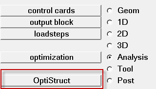
Figure 7. Accessing the OptiStruct Panel
View the Results
-
On the toolbar, click
 (Contour).
-
Under Result type, from the second drop-down menu, select
vonMises.
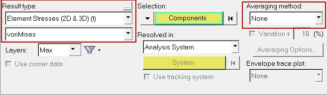
Figure 8. Contour Panel -
Verify that the fields in the Contour panel match those in
Figure 8 and click
Apply.
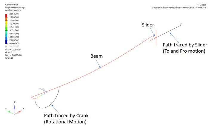
Figure 9. Contour of Displacement in Crank Slider model. Time = 0.98 sec