Seam Weld Fatigue (FPM) using S-N Method

The method is a hot-spot stress approach applicable to thin metal sheets.

Hot-spot stress is calculated from grid point forces at the weld line. The method showed a good agreement with laboratory test results for sheet thickness between 1.0 mm and 3.0 mm. The method typically requires two SN curves. One is a bending SN curve which is dominated by bending stress, and the other is a membrane SN curve which dominated by membrane stress.

The following file found in the optistruct.zip file is needed to perform this tutorial. Refer to Access the Model Files.

SeamWeld_frame.fem

or

A copy of the model files used in this tutorial are available on <install_directory>/tutorials/hwsolvers/optistruct.

In this tutorial, a frame is experiencing frontal and rear torsional loads in addition to vertical bending. Seam Welds are modeled between the sections forming the frame.


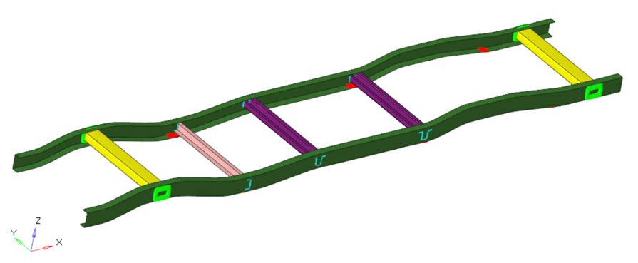
Figure 1. Automotive Frame
You will be able to calculate the damage that occurs at the seam (fillet) welds modeled. The solver deck setup is done using process manager. The following contents are covered:
  • Launch Fatigue Process Manager
  • Import a model
  • Create fatigue subcase
  • Define fatigue analysis parameters
  • Define fatigue elements and S-N properties
  • Define load-time history and loading sequence
  • Submit the job
  • View results summary and launch HyperView for post-processing

Launch HyperMesh and Set the OptiStruct User Profile

The model being used for this exercise is that of an automotive frame (Figure 1). The input file consists of 3 static loadsteps to which the frame is subjected to – Frontal torsion, Rear torsion and the Vertical bending.

  1. Launch HyperMesh.
    The User Profile dialog opens.
  2. Select OptiStruct and click OK.
    This loads the user profile. It includes the appropriate template, macro menu, and import reader, paring down the functionality of HyperMesh to what is relevant for generating models for OptiStruct.
  3. Click Tools > Fatigue Process > Create New.
  4. For New Session, enter a name in your working directory folder.
  5. Click Create.
    This creates a new file to save the instance of the currently loaded fatigue process template.

Import the Model

  1. Click File > Import > Solver Deck.
    An Import tab is added to your tab menu.
  2. For the File type, select OptiStruct.
  3. Select the Files icon files_panel.
    A Select OptiStruct file browser opens.
  4. Select the SeamWeld_frame.fem file you saved to your working directory. Refer to Access the Model Files.
  5. Click Open.
  6. Click Import, then click Close to close the Import tab.
    The outline of the Fatigue Analysis setup to be achieved in the following steps.


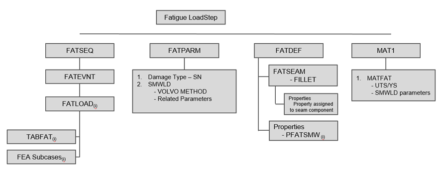
    Figure 2. Fatigue Setup - Fillet Seam Welds

Set Up the Model

Create a Fatigue Subcase

  1. Make sure the task Fatigue Subcase is selected in the Fatigue Analysis tree.
  2. In the Create new fatigue subcase field, enter Fatigue_3LCs_SeamWeld.
  3. Click Create.
  4. For the Select existing fatigue subcase field, select the newly created fatigue subcase Fatigue_3LCs_SeamWeld.
    Fatigue_3LCs_SeamWeld is selected as the active fatigue subcase. Definitions in the following processes (analysis parameters, fatigue elements and properties, loading sequences, etc.) will be for this subcase.
  5. Click Apply.
    This saves the current definitions and guides you to the next task Analysis Parameters of the Fatigue Analysis tree.


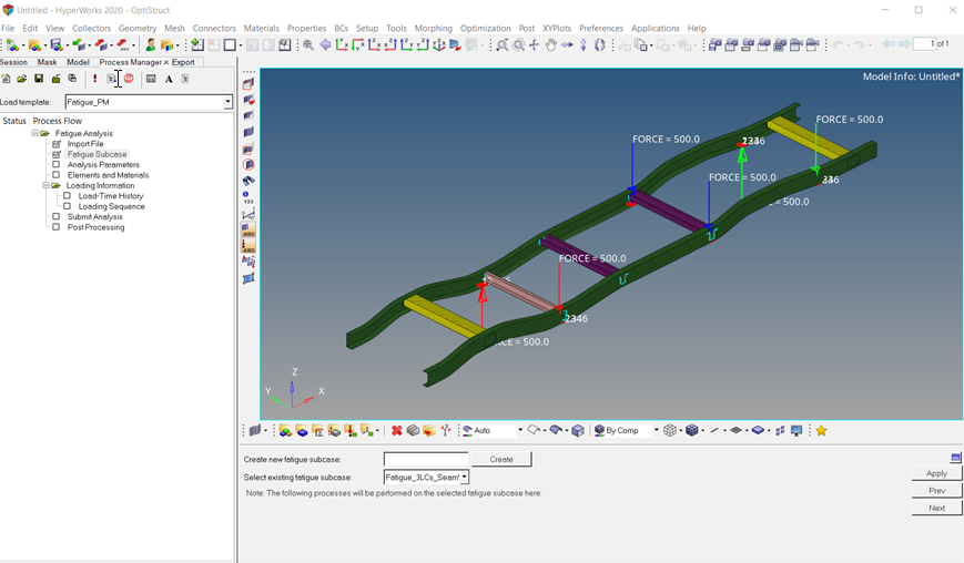
    Figure 3. Create and Select Active Fatigue Subcase to Process

Define Fatigue Parameters

  1. In the Model Browser, right-click and select Create > Load Collector.
  2. For Name, enter fatparam.
  3. For Card Image, select FATPARM.
  4. Verify TYPE is set to SN.
  5. Set STRESS COMBINE to SGVON (Signed von Mises).
  6. Set STRESS CORRECTION to GERBER.
  7. Set STRESSU to MPA (Stress Units).
  8. Set RAINFLOW RTYPE to LOAD.
  9. Set GATEREL to 0.0.
  10. Set CERTNTY SURVCERT to 0.5.
  11. Check the box beside SMWLD and select the following options:

    METHOD = VOLVO

    Mean Stress Connection = FKM

    SURVCERT = 1e-9

    THCKCORR = YES

  12. Click Apply.
    This saves the current definitions and guides you to the next task Elements and Materials of the Fatigue Analysis tree. For details, refer to the Altair Simulation 2022 help.

Add Fatigue Elements and Materials

Make sure the task Elements and Materials is selected in the Fatigue Analysis tree.

  1. Click Add Material.
    A Material Data window opens.


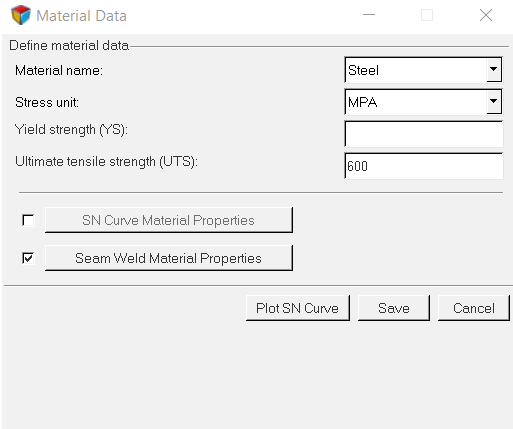
    Figure 4. Material Data Definition
  2. For Material name, select Steel.
  3. Make sure Stress unit is set to MPA.
  4. For Ultimate tensile strength (UTS), enter 600.
  5. Activate Seam Weld Material Properties, then click Seam Weld Material Properties.
  6. Enter the values for Mean Stress Sensitivity, MSS2, Structural SN Curve along with bending and membrane SN curve material values, as shown below.


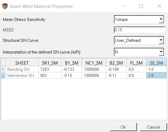
    Figure 5. Seam Weld Material Properties dialog
  7. Click OK.
  8. Click Save.
  9. Click Add Property.


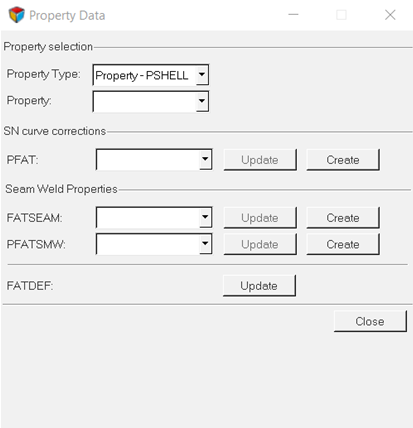
    Figure 6. Property Data dialog
  10. For Property Type, select Property - PSHELL.
  11. Click Close to save the definition of the SN data for the selected property.

Define PFATSMW Property

BRATIO helps understand if the Bending Moments or if the Membrane Forces dominates the maximum stresses based on which the interpolated SN curve is created.

Similarly, TREF and TREF_N help in accounting for thickness correction

  1. In the Model Browser, right-click and select Create > Property.
  2. For Name, enter PFATSMW_7.
  3. For Card Image, select PFATSMW.
  4. Set BRATIO to 0.6.
  5. Set TREF to 1.1.
  6. Set TREF_N to 0.1.
  7. Click Close.

Define FATDEF Load Collector

  1. In the Model Browser, right-click and select Create > Load Collector.
  2. For Name, enter FATDEF1.
  3. Set the Card Image to FATDEF.
  4. Activate FATSEAM in the PTYPE Entity Editor.
  5. For FATDEF_FATSEAM_NUMIDS, enter 1.
  6. Select FatSeam for FATSEAMID and PFATSMW_7 for PFATSMWID.
  7. Click Close.

Apply Load-Time History

  1. Make sure the task Load-Time History is selected in the Fatigue Analysis tree.
  2. Click Add by File.
    A Load Time History window opens.
  3. For Load-time history name, enter LTH1.
  4. For Load-time history type, select CSV.
  5. Click the Open load-time file icon files_panel.
    An Open file browser window opens.
  6. Browse for load1.csv.
  7. Click Open > Import.
  8. Click Save to write the new load-time history into HyperMesh database.
  9. Create another load-time history LTH2 by importing the file load2.csv.
  10. Click Plot L-T to show the load-time history.
  11. Close the Load Time History window.
  12. Click Apply.
    This saves the current definitions and guides you to the next task Loading Sequences of the Fatigue Analysis tree.
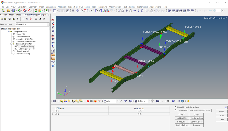

    Figure 7. Load-Time History Definition
    Note: The RPC/RSP and DAC file formats are now supported in fpm. Make sure to use HyperMesh Desktop application for this.

Load Sequences

In this step, one event consisting of two load time history is created; in other words, the linear superposition of the stress caused by the two load time history is requested during analysis. Using this event, one load sequence is constructed.
  1. Make sure the task Loading Sequences is selected in the Fatigue Analysis tree.
  2. Click Add.
    A Load Mapping window opens.
  3. Activate the radio button Manual and leave the event creation method set to default Single Event.
  4. Click + button to create a single event with three subcases and two channels.
  5. Drag and drop the three subcases (Front Torsional Stiffness, Rear Torsional Stiffness and Vertical Bending Stiffness) under Subcases of the newly created event.
  6. Drag and drop the two channels (LTH1 and LTH2) to the three subcases to create loading sequence, as shown below.
  7. Drop LTH1 for the first subcase (Front Torsional Stiffness) and LTH2 for the other two subcases (Rear Torsional Stiffness and Vertical Bending Stiffness).
  8. Set LDM to 0.1 and Scale to 0.6 for all three cases.


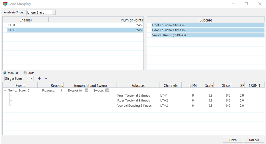
    Figure 8. Load Mapping to associate load-time history with static subcase
  9. Click Save to close the window and create the fatique event using selected subcases and channels.


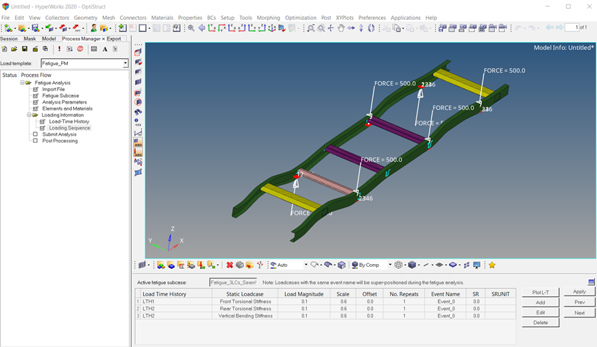
    Figure 9. Loading Sequences Definition

Submit the Job

Make sure the task Submit Analysis is selected in the Fatigue Analysis tree.

  1. From the Analysis page, enter the OptiStruct panel.
  2. Click save as following the input file field.
    The Save As dialog opens.
  3. For File name, enter the name seamweld_frame_fat.fem.
  4. Click Save twice.
  5. For Run Option, select analysis.
  6. Click Submit.
    This launches OptiStruct to run the fatigue analysis.
    If the job was successful, new results files can be seen in the directory where the OptiStruct model file was written. The default files written to your directory are:
    seamweld_frame_fat.h3d
    Hyper 3D binary results file, with both static analysis results and fatigue analysis results.
    seamweld_frame_fat.out
    OptiStruct output file containing specific information on the file set up, the set up of your fatigue problem, compute time information, etc. Review this file for warnings and errors.
    seamweld_frame_fat.stat
    Summary of analysis process, providing CPU information for each step during analysis process.

Post-process the Analysis

  1. Make sure the task Post-processing is selected in the Fatigue Analysis tree.
    When fatigue analysis has completed successfully after the previous submit, it will automatically go into this task.
  2. For Fatigue subcase, make sure Select Subcase is selected.
  3. For Result Type and Data Component, select the required data you want to contour from the drop-down menu.
  4. Click Load H3D Results (HV).
    This launches HyperView and loads the seamweld_frame_fat.h3d results file. It applies the result contour for selected result type and component. You can use HyperView for more detailed results.
  5. Click Exit to unload Fatigue Process Manager.


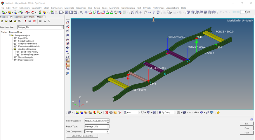
    Figure 10. Post-Processing


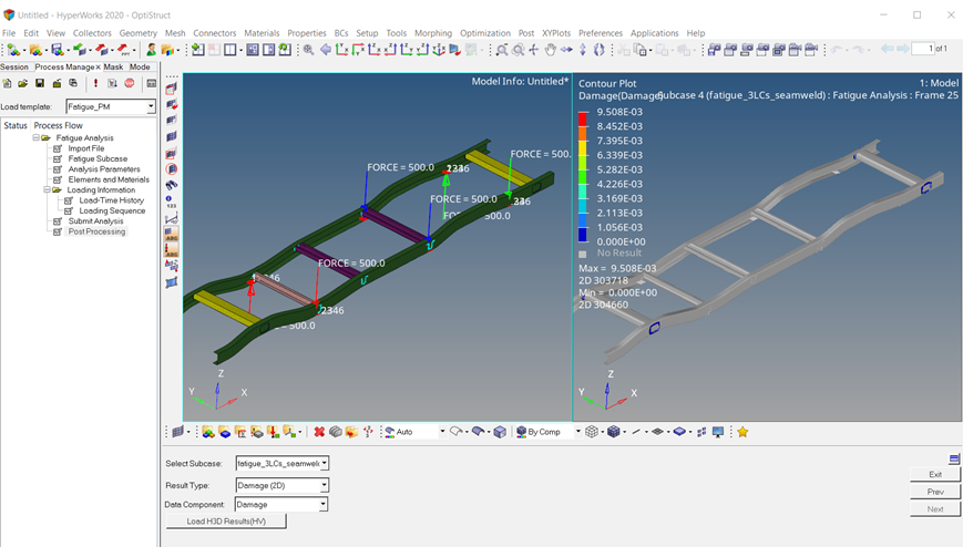
    Figure 11. Damage Contour in HyperView