OS-T: 3010 Topography Optimization of an L-bracket
In this tutorial you will perform a topography optimization on a L-bracket modeled
with an attached mass.
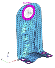
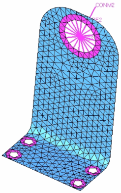
The bracket is modeled with shell elements. The objective is to maximize the
frequency of the first mode by introducing beads or swages to the bracket. This can
be achieved by using topography optimization. The regions around the holes are
specified as non-designable, while the bulk of the bracket is available for
developing stiffening beads. Figure 1. L-bracket Layout
The optimization problem for this tutorial is stated as:
Objective
Maximize 1st frequency mode.
Constraints
Bead dimensions and layout.
Design Variables
Perturbation of nodes normal to the shell's mid-plane.
Launch HyperMesh and Set the OptiStruct User Profile
Launch HyperMesh.
The User Profile dialog opens.
Select OptiStruct and click
OK.
This loads the user profile. It includes the appropriate template, macro
menu, and import reader, paring down the functionality of HyperMesh to what is relevant for generating models for
OptiStruct.
Open the Model
Click File > Open > Model.
Select the Lbkttopog.hm file you saved to
your working directory from the optistruct.zip file. Refer
to Access the Model Files.
Click Open.
The Lbkttopog.hm database is loaded
into the current HyperMesh session, replacing any
existing data.
Set Up the Optimization
Define Topography Design Variables
For a topography optimization, a design space and a bead definition need to be
defined.
In this step, the values of a bead width of 15mm, a bead height of
5mm, and draw angle of 85 degrees will be used. Symmetry of the bead pattern should
be forced along the symmetry line of the design space.
From the Analysis page, click the optimization
panel.
Click the topography panel.
Create a topography design space definition.
Select the create subpanel.
In the desvar= field, enter topo.
Using the props selector, select design.
Click create.
A topography design space definition, topo,
has been created. All elements organized into the design component collector(s) are now included in the design space.
Create a bead definition for the design space topo.
Select the bead params subpanel.
Verify the desvar = field is set to topo,
which is the name of the newly created design space.
In the minimum width= field, enter 15.0.
This parameter controls the width of the beads in the model. The
recommended value is between 1.5 and 2.5 times the average element
width.
In the draw angle= field, enter 85.0 (this is the
default).
This parameter controls the angle of the sides of the beads. The
recommended value is between 60 and 75 degrees.
In the draw height=, enter 5.0.
This parameter sets the maximum height of the beads to be
drawn.
Select buffer zone.
This parameter establishes a buffer zone between elements in the
design domain and elements outside the design domain.
Toggle draw direction to normal to
elements.
This parameter defines the direction in which the shape variables are
created.
Set boundary skip to load and spc.
This tells OptiStruct to leave nodes at
which loads or constraints are applied out of the design space.
Click update.
A bead definition has been created for the design space topo. Based on this information, OptiStruct will automatically generate bead variable
definitions throughout the design variable domain.
Adding pattern grouping constraints.
Select the pattern grouping subpanel.
Click desvar = and select topo.
Set the pattern type to 1-pln sym.
Click anchor node, and enter 337 in the id=
field.
Click first node, and enter 613 in the id= field.
Click update.
Update the bounds of the design variable.
Select the bounds subpanel.
Verify the desvar = field is set to topo,
which is the name of the design space.
In the Upper Bound= field, enter 1.0.
Upper bound on variables controlling grid movement (Real > LB, default
= 1.0). This sets the upper bound on grid movement equal to
UB*HGT.
In the Lower Bound= field, enter 0.0.
Click update.
The upper bound sets the upper bound on grid movement equal to UB*HGT
and the lower bound sets the lower bound on grid movement equal to
LB*HGT.
Click return to go to the Optimization panel.
Create Optimization Responses
From the Analysis page, click optimization.
Click Responses.
Create the frequency response.
In the responses= field, enter FREQ.
Below response type, select frequency.
For Mode Number, enter 1.0.
Click create.
A response, FREQ, is defined for
the frequency of the first mode
extracted.
Click return to go back to the Optimization panel.
Define the Objective Function
Click the objective panel.
Verify that max is selected.
Click response and select FREQ.
Using the loadsteps selector, select STEP.
Click create.
Click return twice to exit the Optimization panel.
Save the Database
From the menu bar, click File > Save As > Model.
In the Save As dialog, enter Lbkttopog.hm for the file name and save it to your
working directory.
Run the Optimization
From the Analysis page, click OptiStruct.
Click save as.
In the Save As dialog, specify location to write the
OptiStruct model file and enter
Lbkttopog for filename.
For OptiStruct input decks,
.fem is the recommended extension.
Click Save.
The input file field displays the filename and location specified in the
Save As dialog.
Set the export options toggle to all.
Set the run options toggle to optimization.
Set the memory options toggle to memory default.
Click OptiStruct to run the optimization.
The following message appears in the window at the completion of the
job:
OPTIMIZATION HAS CONVERGED.
FEASIBLE DESIGN (ALL CONSTRAINTS SATISFIED).
OptiStruct also reports error messages if any exist. The
file Lbkttopog.out can be opened in a
text editor to find details regarding any errors. This file is written to the
same directory as the .fem file.
Click Close.
The default files that get written to your run directory include:
Lbkttopog.hgdata
HyperGraph file containing data for the
objective function, percent constraint violations, and constraint for
each iteration.
Lbkttopog.hist
The OptiStruct iteration history file
containing the iteration history of the objective function and of the
most violated constraint. Can be used for a xy plot of the iteration
history.
Lbkttopog.html
HTML report of the optimization, giving a
summary of the problem formulation and the results from the final
iteration.
Lbkttopog.oss
OSSmooth file with a default density threshold of 0.3. You may edit the
parameters in the file to obtain the desired results.
Lbkttopog.out
OptiStruct output file containing specific
information on the file setup, the setup of the optimization problem,
estimates for the amount of RAM and disk space required for the run,
information for all optimization iterations, and compute time
information. Review this file for warnings and errors that are flagged
from processing the Lbkttopog.fem file.
Lbkttopog.sh
Shape file for the final iteration. It contains the material density,
void size parameters and void orientation angle for each element in the
analysis. This file may be used to restart a run.
Lbkttopog.stat
Contains information about the CPU time used for the complete run and
also the break-up of the CPU time for reading the input deck, assembly,
analysis, convergence, and so on.
Lbkttopog_des.h3d
HyperView binary results file that contain
optimization results.
Lbkttopog_s#.h3d
HyperView binary results file that contains
from linear static analysis, and so on.
Lbkttopog.grid
An OptiStruct file where the perturbed grid
data is written.
View the Results
Shape contour information is output from OptiStruct for all iterations. In addition,
Eigenvector results are output for the first and last iteration by default.
This section describes how to view those results in HyperView.
View a Transient Animation of Shape Contour Changes
From the OptiStruct panel, click HyperView.
HyperView launches within the HyperMesh Desktop and loads the Lbkttopog_des.h3d file.
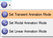
On the Animation toolbar, set the animation mode to
Transient.
Figure 2.
Click to start the animation.
Click to open the Animation Controls panel.
Move the Max Frame Rate slider to adjust the animation speed.
Review the Optimized Frequency Difference
In the top, right of the application, click to proceed page 3, which contains the results for first and the last
iterations.
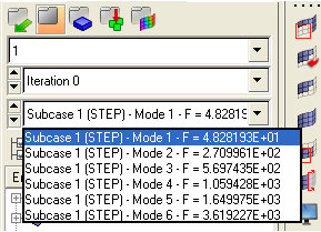
In the Results Browser, select the first iteration
(Iteration 0).
The frequencies of all of the modes requested from the analysis are shown in the
Subcase drop-down. Figure 3. Frequency of the First Mode for Iteration 0
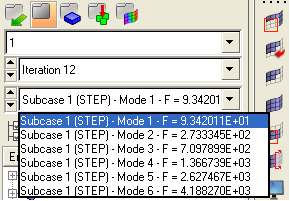
Look at the frequency values for the last iteration. Upon observation, the frequency
for the first mode has changed from around 48 Hz to around 93 Hz for first and last
iterations, respectively. Figure 4. Frequency of the First Mode for Iteration 12
Apply Optimized Topography
In the top, right of the application, click to go back to the Design History page (page 2).
On the Animation toolbar, click to set the Current time to the last
step.
 to start the animation.
 to open the Animation Controls panel.
 to proceed page 3, which contains the results for first and the last
iterations.
to proceed page 3, which contains the results for first and the last
iterations.
 to set the Current time to the last
step.
to set the Current time to the last
step.