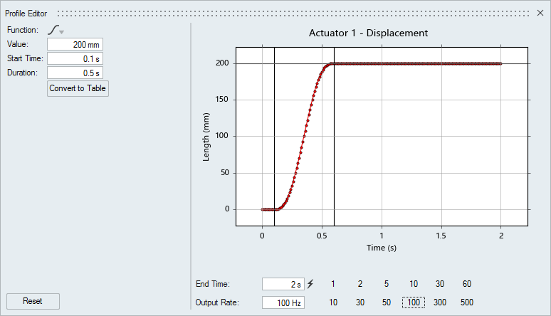
Use the Profile Editor to view and edit profile functions.
Change the profile function.
Change the parameters of the currently selected profile, such as the value,
start time, and duration.
Modify the profile data interactively in the chart.
Convert the profile to a table and save it as a .csv file.
View the Profile Editor (Time Dependent)
Click on the motors or actuators microdialog
to open the Profile Editor.
Figure 1. Profile Editor
Tip:
If you enter zero for the Value, the motor or actuator will be locked and
the Profile Editor will become uneditable. To reverse this, double-click the
motor or actuator in the modeling window to edit it, and click on the microdialog to unlock it
Click the Reset button to restore the current profile
function to its default values
Certain profile functions have sliders under some parameters. You can click
and drag a slider to shape the profile function.
Right-click on the plot and then click Export Image
to export an image of the profile function.
Look closely at the Start Time setting when changing
back and forth between profiles or when using the Convert to
Table option.
Modify the Profile Function Interactively (Time Dependent)
Click and drag the plot sliders in the Profile Editor to reshape the profile
function.
Sliders are highlighted as you hover over them with the mouse, and a memory
curve shows the original shape.
The sliders can snap to grid lines or parameters on other profile functions.
Press Alt to temporarily disable snapping.
Blue dashed lines, when visible, represent other profiles in use in the model.
You can snap to features on those profiles as well.
Tip:
You can pan, zoom, and fit the plot. When zooming, use the
Ctrl key to keep the x-axis fixed. Press
F or double-click to fit the plot.
Clicking on the plot sliders also puts focus on the associated property.
This makes it easy to gain more precise control by typing in a value.
For table functions, click and drag data points in the chart to modify them
individually. You can also box select to move multiple data points
simultaneously.
To provide better control when adjusting curves, the tool tip for time-based
sliders shows the absolute time.
When your time unit is milliseconds, the Output Rate reports the value in
kHz.
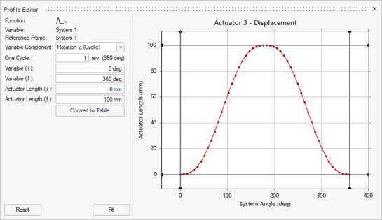
Specify the Variable Range or Cycle (State Dependent)
In the Profile Editor, specify the variable range or cycle over which the input
function will be applied.
Option
Description
Function
Select a profile function. Supported functions include:
Step
Step Dwell Step
Single Wave
Impulse
Table
Variable
The independent variable object (system, measure, motor, or
actuator).
Reference Frame
The reference frame used by the variable component.
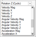
Variable Component
The independent variable component output that the state
dependent object will monitor. Use the dropdown menu to access
to the library of functions.
One Cycle (for cyclic
rotations)
Specify the cycle range within which the V(i) and V(f) values
fall. For example, a 4-stroke piston engine will experience
combustion force every 2 revolutions (or 720 degrees) of the
crankshaft.
Variable (i)
Enter the initial value of the independent variable object
(system, measure, motor, or actuator).
Variable (f)
Enter the final value of the independent variable object
(system, measure, motor, or actuator).
[Variable Object] Force (i)
Enter the initial value of the state dependent
object.
[Variable Object] Force (f)
Enter the final value of the state dependent object.
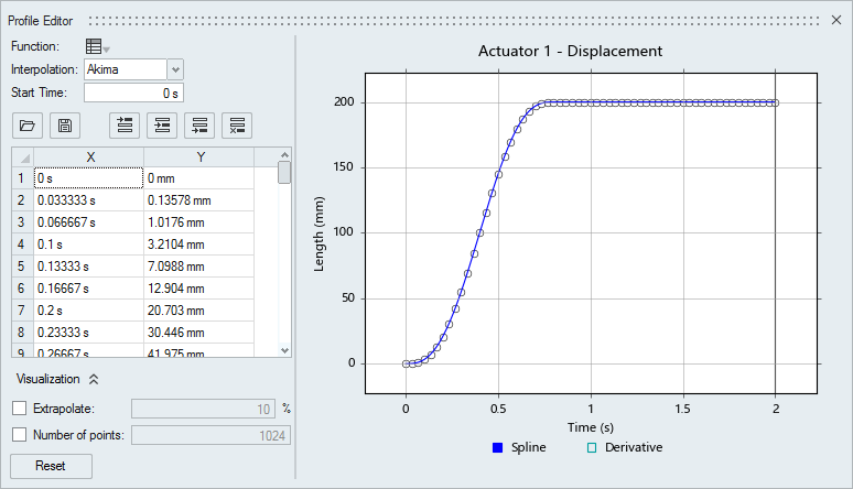
Convert a Profile Function to a Table
Convert a profile function to a table to modify data points and save them in a .csv
file.
Select the Table function to convert a profile function to a table. Click
Spline or Derivative in the legend
to plot one or the other.
Figure 2. Profile Function Converted to a Table
Option
Description
Load values from a .csv file. Alternatively, you can drag and
drop a valid .csv file onto the profile editor.
Save data to a .csv file.
Insert a value before the first data point.
Insert a value after the selected data point.
Insert a value after the last data point.
Delete the selected data points.
Extrapolate
Linearly extrapolate the curve at both ends. The default is
10%.
Number of points
The number of interpolation points. The default is 1024 points.
If the Spline curve does not appear to be passing through your data
points, try increasing the Number of Points
under the Visualization section.
Shortcuts
To
Do This
Disable snaps temporarily
Press Alt
Pan the plot
Click and drag the right mouse button.
Zoom in the plot
Use the scroll wheel on the mouse. Press Ctrl
+ scroll to keep the x-axis fixed (zoom y). Press Shift
+ scroll to keep the y-axis fixed (zoom x).
 on the motors or actuators microdialog
to open the Profile Editor.
on the motors or actuators microdialog
to open the Profile Editor.
 on the microdialog to unlock it