Example 14: 51x51 Array Physical Antenna with Radome Using Dolph-Chebychev Algorithm

This case explains how to use the Dolph-Chebychev algorithms to calculates the pointing parameters in a bidimensional coaxial feed array, to which a radome is added.

Step 1 Create a new MoM Project.

Open newFASANT and select File - New option.

Figure 1. New Project panel

Select MOM option on the previous figure and start to configure the project.

Step 2 Set the simulation parameters as shown.

Select Simulation - Parameters option, set the parameters and save it.

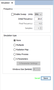
Figure 2. Simulation panel

Step 3 Create the array

First, select 'millimeters' on units list on the bar at the bottom of the main window.

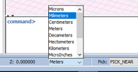
Figure 3. The first element is created using Source - Coaxial Feed - Add Feed Point.

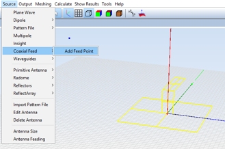
Figure 4. Add feed point

Select the surfaces and click on Add.

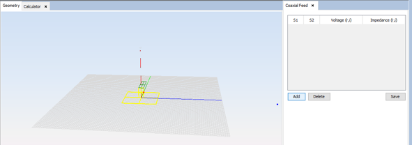
Figure 5. Coaxial Feed panel

Then save the feed point.

Use the array command and enter the characteristics of the array.

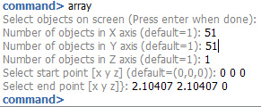
Figure 6. Array parameters

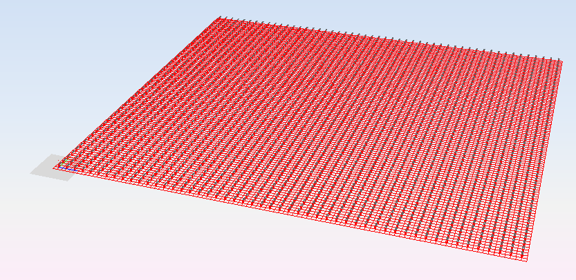
Figure 7. Array view

Step 4 Create the radome

The radome will be made of two concentric hemispheres that will be put over the array. In order to make a hemisphere, first create a sphere, using the sphere command.

Figure 8. Sphere parameters

Select the sphere in the objects tree and use the explode command.

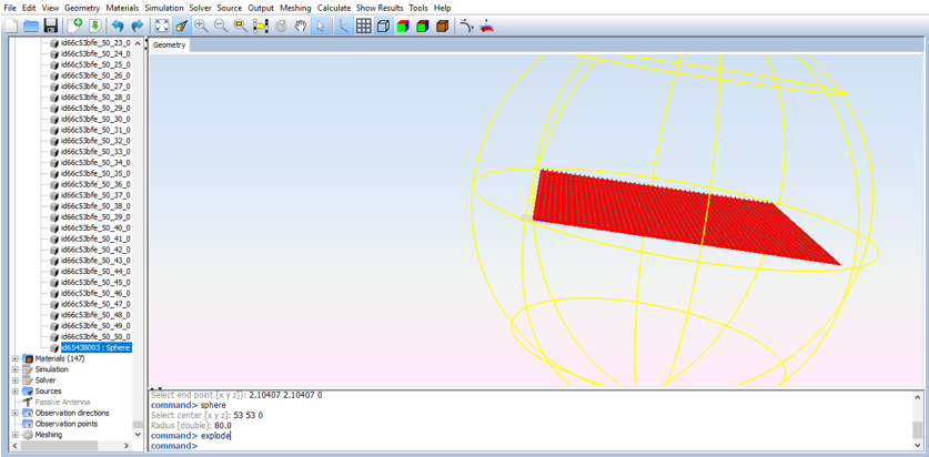
Figure 9. Sphere selection and explode command

Select the four bottom surfaces and execute 'delete' command. Then the surfaces will be removed from the geometry.

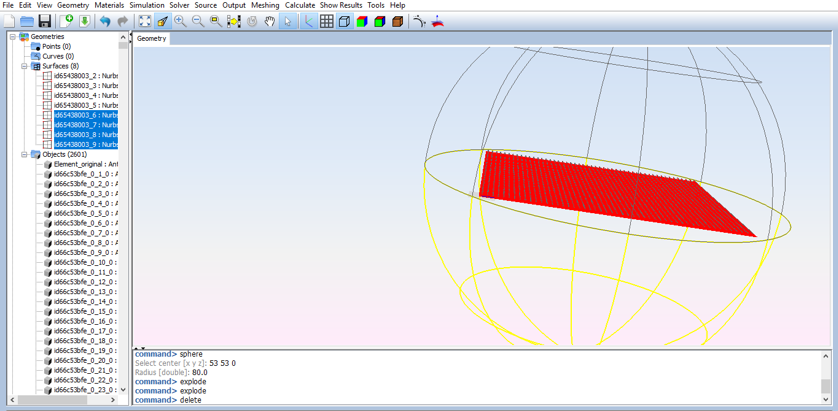
Figure 10. Surface selection and delete command

Select all remaining surfaces and execute group command.

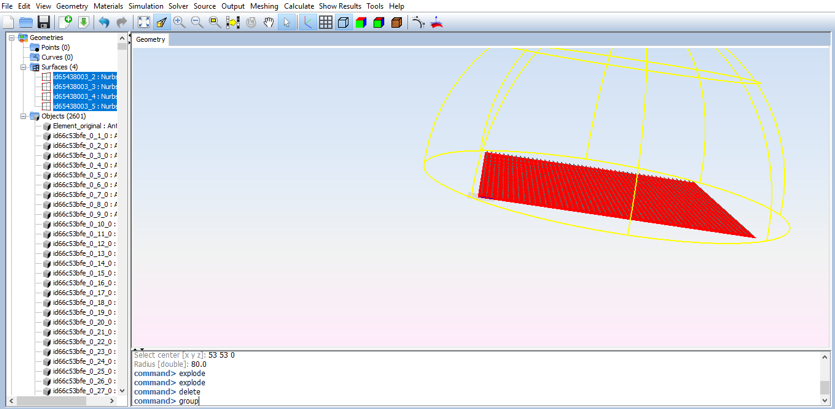
Figure 11. Surfaces selection and group command

Now that the hemisphere is done, create another one following the same steps, but with a bigger radius.

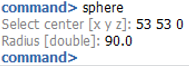
Figure 12. Sphere parameters.

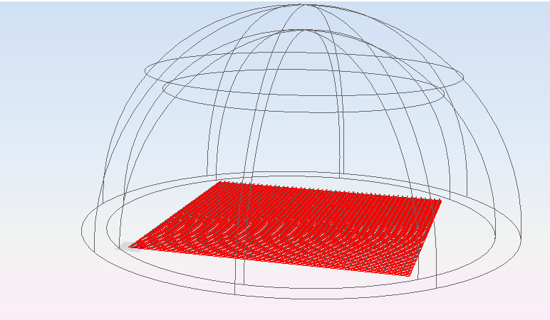
Figure 13. Project view

To create the radome, click on Source - Radome - Define Radome. Click on the button Add Radome.

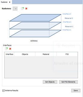
Figure 14. Radome panel

Select the inner semi-sphere as the first interface and click on Set Objects.

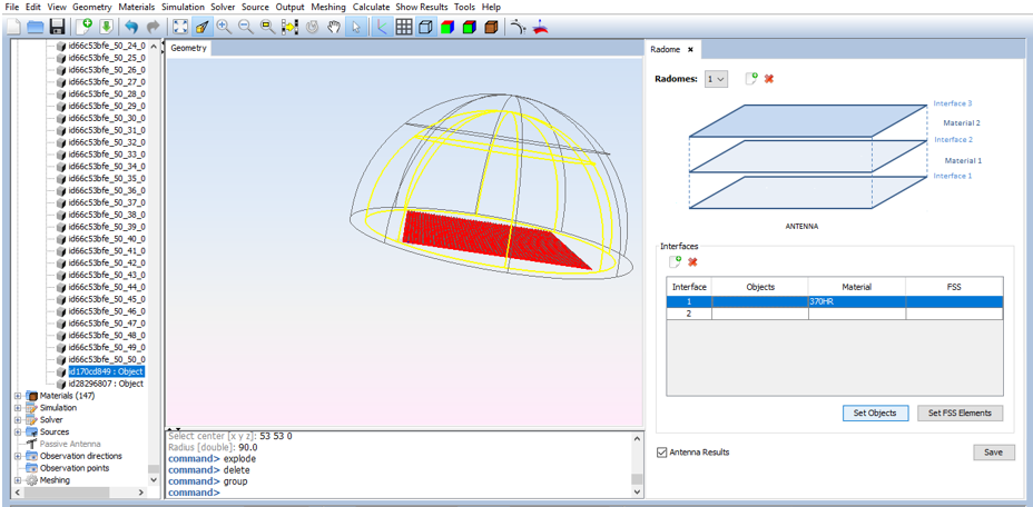
Figure 15. Radome panel

Then, select the outer semi-sphere as the second interface.

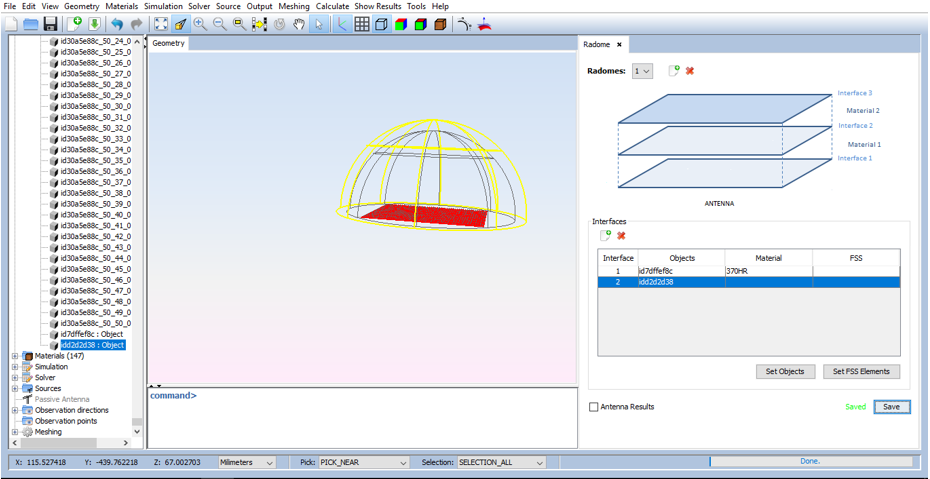
Figure 16. Radome panel

Save the parameters of the radome.

Step 5 Feed the array

To set the feeding of the array select Source - Antenna Feeding and the following panel will open.

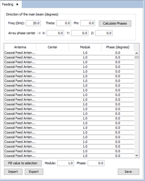
Figure 17. Antenna Feeding panel

This is the default setting. To use the Dolph-Chebychev algorithm click on Tools - User Function and select the corresponding function. NOTE To use the bidimensional Dolph-Chebychev function it is needed to download both the bidimensional and the unidimensional functions.

Figure 18. Bidimensional Dolph-Chebychev function

A path has been selected by default so the files will be created on the mydatafiles folder in the newFASANT directory.

Figure 19. Bidimensional Dolph-Chebychev function

The next step is generating the text file. To do so click on Tools - Calculator and write the call to the function.

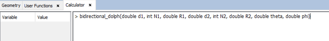
Figure 20. Calculator panel

In this case, set the parameters as shown. Angles of theta=20º and phi=45º, and a side lobe level of 50dB are selected as an example.

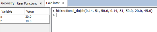
Figure 21. Calculator panel

A spacing of 0.14 in units of lambdas is selected because is equivalent to a spacing of 2.104 millimeters at 20 GHz.

The text file will be automatically generated in the mydatafiles folder.

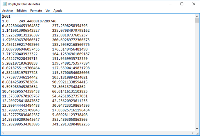
Figure 22. Results file

Now, apply these results to the array created before by clicking on Source - Antenna Feeding.

The panel shown before will appear. To use the weights and phases calculated with the Dolph-Chebychev algorithm, click on Import.

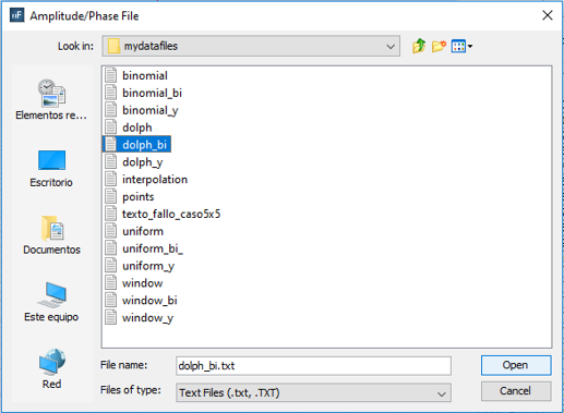
Figure 23. Amplitude/Phase File panel

Select the corresponding file and save the feeding.

Step 6 Solver parameters

Select Solver - Advanced Options and set the parameters as shown.

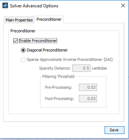
Figure 24. Solver Advanced Options panel

Step 7 Meshing the geometry model.

Select Mesh - Create Mesh to open the meshing configuration panel and then set the parameters as show the next figure.

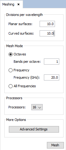
Figure 25. Meshing panel

Click on Mesh.

Step 8 Execute the simulation.

Select Calculate - Execute option to open simulation panel.

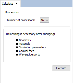
Figure 26. Calculate panel

Step 9 Show Results.

The radiation cuts can be visualized by clicking on Show Results - Radiation Pattern - View Cuts.

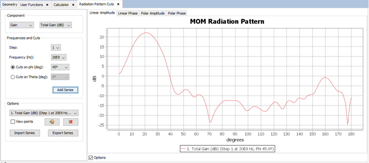
Figure 27. Radiation Pattern Cuts

Note that the side lobe level selected earlier must be represented here.

Here is a comparison of this example with a project that has the same array but without the radome. The blue line represents the array with the radome and the red line is the project without radome.

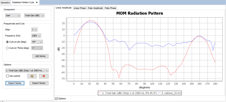
Figure 28. Radiation Pattern Cuts

The radiation pattern can be visualized by clicking on Show Results - Radiation Pattern - View 3D Pattern.

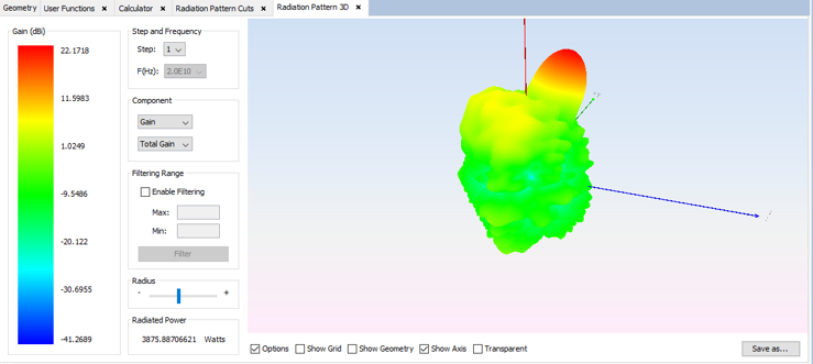
Figure 29. Radiation Pattern 3D