Advanced Solver Options
As covered before, it is possible to set the Solver Functions when the solver method has been set to MoM. Solver functions have custom settings that can be changed by selecting the Advanced Options button in the Solver Functions. Pressing this button shows a dialog with two visible tabs:
- Main Properties: this tab has settings for changing how the solver works, including which kind of algorithm will the solver use.
- Preconditioner: this tab contains available preconditioners for the selected solver.
- CBFs Properties: this tab is only enabled when the solver functions are set to CBFs.
The Main Properties tab looks like this:
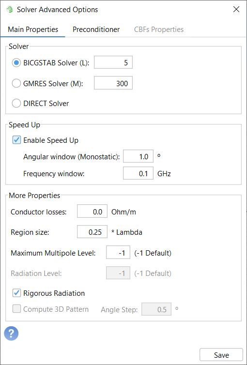
Figure 1. Main Properties
The following settings are available:
-
Solver: Three algorithms to solve the problem are available. We can choose between two iterative methods, like BICGSTAB (BiConjugate Gradient STAbilized method) and GMRES (Generalized Minimal Residual method), and the DIRECT solver. If no convergence is achieved by using any of the iterative methods, it is recommended to try to use the other one.
Direct Solver improves the efficiency in time when the problem is less than the number of unknowns introduced. Direct Solver is enabled only if OpenMP Architecture is selected on the main Solver window, and is not compatible with Speed Up and preconditioners.Note: The direct solution method may require huge memory and time resources when a large number of unknowns is considered. - Speed Up: If the user enables the speed-up, this option reduces the analysis time for problems that have several incident angles at different frequencies.
- More Properties: This group lets the user set other special parameters used by the solver, such as the conductor losses, region size or maximum multipole level. Rigorous Radiation improves efficiency of the solved solution, but is not compatible with the 3D Radiation computation. The 3D Radiation computation is not compatible with Monostatic RCS.
The Preconditioner tab contains the following options:
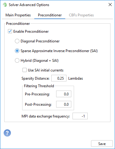
Figure 2. Preconditioner
This tab mainly covers the usage of the Preconditioner, which speeds up the resolution of the problem by selecting one of the possible preconditioners provided.
- Diagonal Preconditioner
- Use this preconditioner only when the mesh density is 10 div/lambda or higher.
- Sparse Approximate Inverse Preconditioner (SAI)
-
- Use SAI initial currents: This option set the currents computed using the SAI preconditioner as the inicial vector of the iterative method. It may be useful if not convergence is achieved in the solution of the problem.
- Sparsity Distance: Set this parameter between 0.2 and 2. Usually hight values increase convergence speed and cpu / memory needs.
- Filtering Threshold: These parameters should contain a value between 0.0 and 1.0. The default values should be adequate in most cases.
- Pre-Processing: This parameter controls the amount of data considered to generate the preconditioner. Lower values entail a more accurate generation, while higher values entail a faster computation.
- Post-Processing: This parameter controls the amount of data to be stored after the generation of the preconditioner. Lower values entail better convergence, while higher values entail less RAM required to store the preconditioner.
- MPI Data Exchange Frequency: This parameter sets up how often the MPI nodes request more coupling terms to generate the preconditioner. Larger values require less interactions speeding up the simulation, although more memory will be needed to store these terms. A negative or 0 value indicates that the coupling terms are only exchanged once.
- Hybrid (Diagonal + SAI)
- This preconditioner is suited for memory-shared machines, in which case will use both Diagonal and SAI preconditioners.
When CBFs are enabled, the following options are available as well:
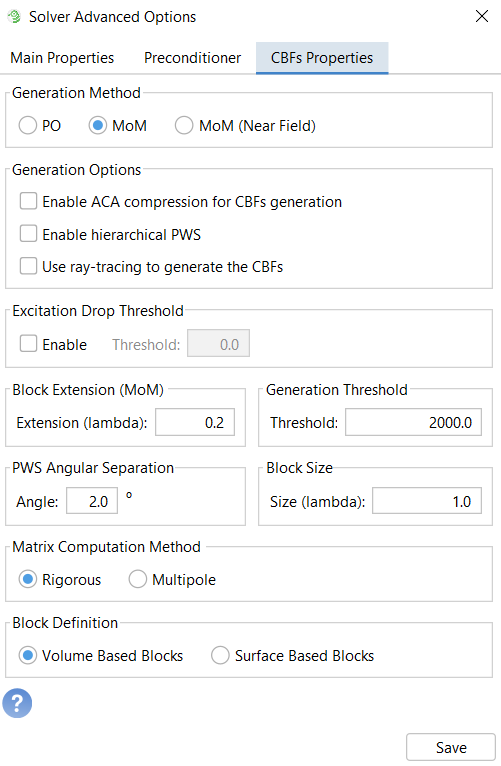
Figure 3. CBFs Properties
These settings let the user configure different parameters of the CBFM method. For most of the analysis, default parameters are suitable.
- Generation method: CBFs can be generated using PO currents or MoM currents (default MoM). In this last option, it is desirable to extend the size of the block to avoid the edge effect. The extension is selected in the Block Extension (MoM) panel (by default, 0.2 lambda).
- Generation Options: There are several techniques that could
speed up the generation of CBF. In this panel, you can select the compression of the
PWS using the ACA technique, the hierarchical computation of the CBFs by dividing the
PWS into groups, or the use of Ray Tracing techniques to establish the number of CBFs
to retain at any block.
- Enable ACA Compression for CBFs generation: This check box enables a compression algorithm using ACA in order to reduce the number of excitations used to obtain the CBFs. This will decrease the total simulation time.
- Excitation Drop Threshold: With this method, a second stage is implemented to discard cbfs. In this case, only CBFs that get a significant impressed field due to external sources are preserved. If used, a threshold of 0.01 is recommended. Lower values give more accuracy.
- Generation Threshold: It is used to set how many cbfs should be retained to solve the problem (Default 2000).
- PWS angular separation: Defines the angular separation between two plane waves in the PWS, which determines how many plane waves will be used in generating the PWS. (By default, 10º).
- Block size: This parameter defines the size of the block of the CBFM method in lambdas.
- Matrix calculation method: You can define the method to calculate the reduced matrix of CBFM, using rigorous calculation or multiple approximation.
- Block definition: This option allow to choose the definition of the block. “Surface-based blocks” define a block that includes only subdomains inside of a MLFMM region that belongs to the same surface. “Volume based blocks” define a block as the set of all subdomains inside of a MLFMM region.
In order to save the solver configuration press the Save button.