In this example, we will calculate the bistatic RCS of an imported geometry using a
frequency sweep from 0.4 GHz to 0.6 GHz.
Step 1
Create a new newFASANT project (using the MONCROS module)
following Step 1 to Step 3 in Example 1.
Step 2
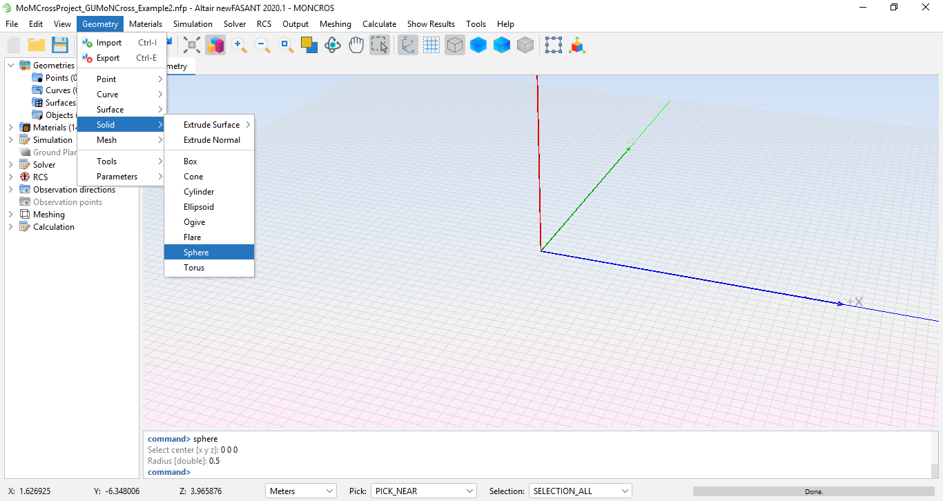
Select Geometry → Solid → Sphere.
Figure 1. Geometry menu
Step 3
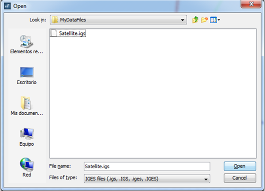
Insert the parameters shown in the figure.
Figure 2. Importing geometry
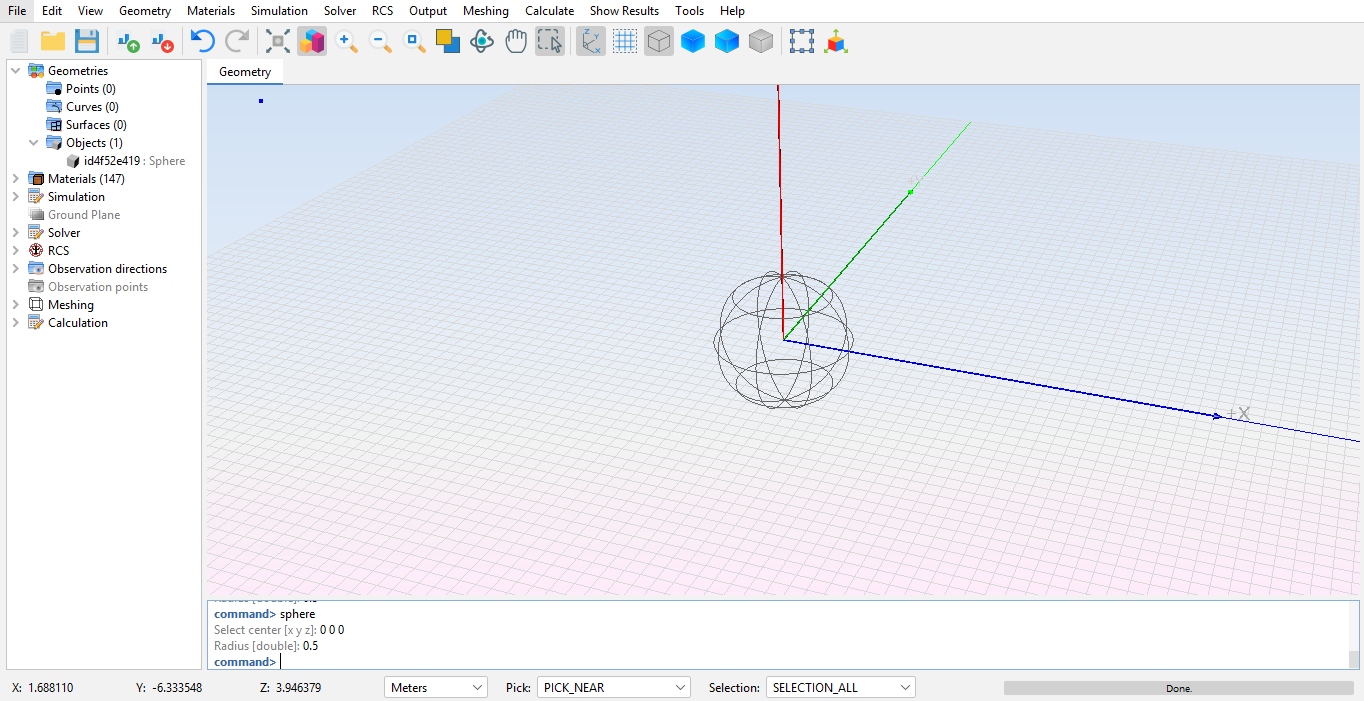
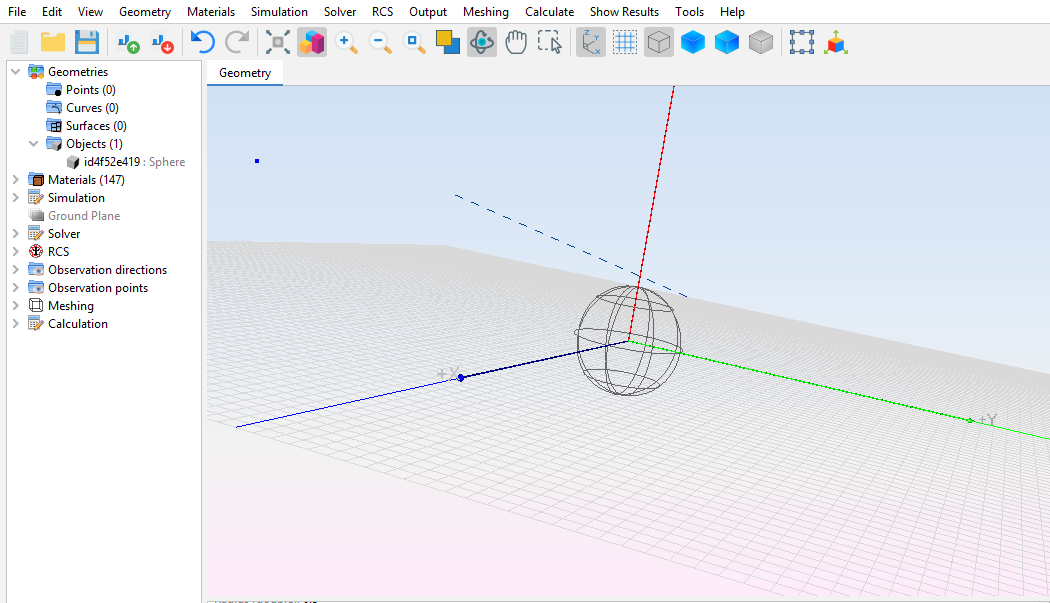
Figure 3. Imported geometry
Step 4
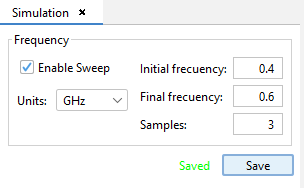
Select the Simulation → Parameters option. Enable the Frequency Sweep option and set
the initial frequency to 0.4 GHz and the final frequency to 0.6 GHz. Set the number
of samples to 3 (the frequencies will be 0.4 GHz, 0.5 GHz and 0.6 GHz) and
left-click the Save button.
Figure 4. Simulation parameters
Step 5
To set up the solver parameters, follow Step 8 of the Example 1 and follow the next
step, making sure to comply with the final warning.
Step 6
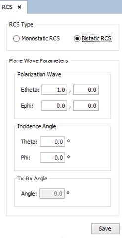
Select the RCS → Parameters option. In the panel that appears, select the Bistatic
RCS option and leave the default values for the remaining options. Press the Save
button.
Figure 5. RCS parameters
WARNING: return to ‘Advanced Options’ of the solver, disable ‘Rigorous Calculate’
option and enable ‘Compute Pattern 3D’ option with the angle value for 0.5 degrees
as default.
Step 7
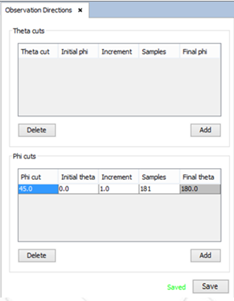
Select the Output → Observation Directions option. Modify the existing phi cut and
set it to 45º. Leave the remaining fields intact. Press the OK button.
Figure 6. Observation Directions panel
Step 8
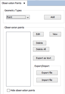
Select the Output → Observation Points option. The following panel will be shown:
Figure 7. Observation Points panel
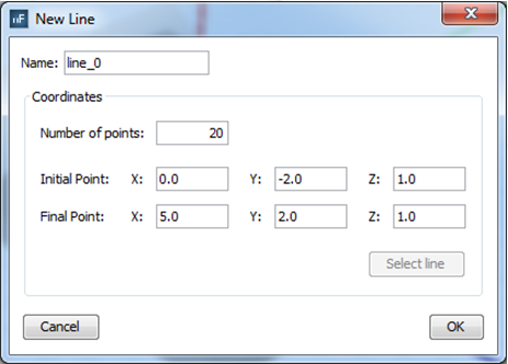
Select the Line option from the Geometry Types combo-box and left-click the Add
button. In the dialog that appears, configure the parameters as shown in the next
figure and press the OK button:
Figure 8. Observation Line parameters
Figure 9. Observation line visualization
Step 9
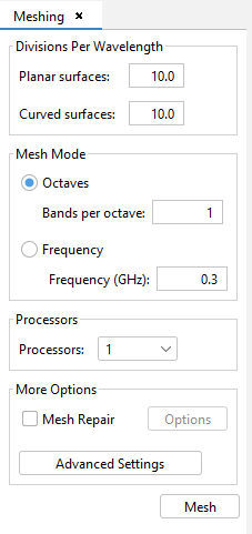
Select Meshing → Create Mesh. Set the options as shown in the following figure:
Figure 10. Meshing options
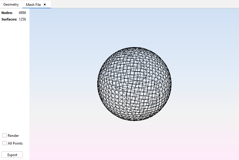
Figure 11. Visualizing the created mesh
Step 10
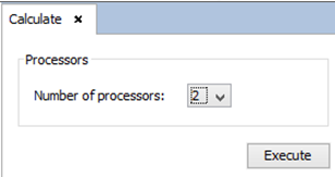
Select Calculate → Execute and set the number of processors that will be used for the
simulation. Press the Execute button to start the simulation.
Figure 12. Calculate options
Step 11
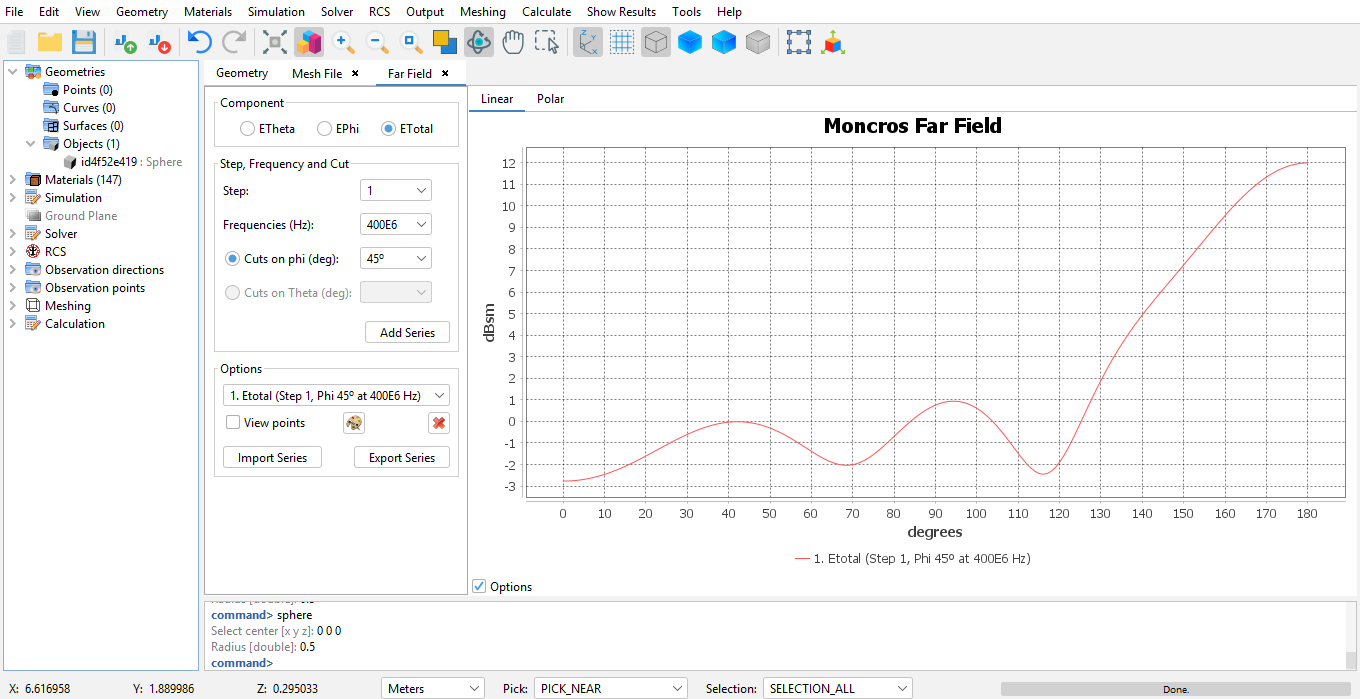
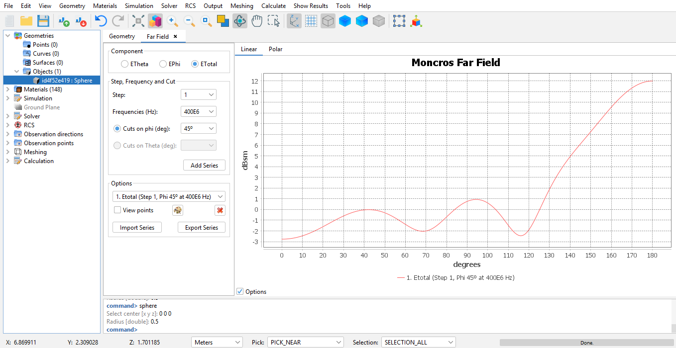
After the simulation finishes, select the option Show Results → Far Field → View
Cuts.
Figure 13. RCS graphic
Initially, only the RCS for the first sampled frequency will be plotted. The user can
add more series by selecting a different frequency in the Frequencies combo-box and
left-clicking the Add Series button.
Step 12
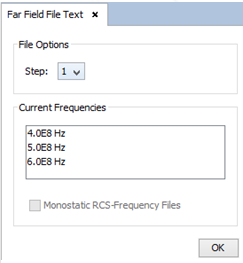
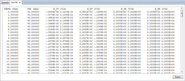
Select Show Results → Far Field → View Text Files. Select the frequency to display
the results for and left-click the OK button.
Figure 14. Far Field Text File options
Figure 15. Viewing RCS results in text format
Step 13
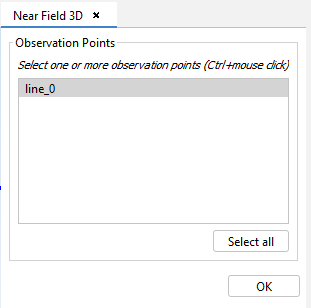
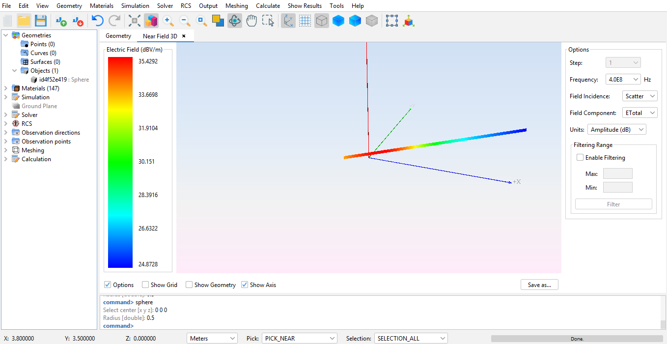
Select the Show Results → Near Field → View Near Field. Select the observation points
to show (in our case, “line_0”) and press the OK button.
Figure 16. View Near Field panel
Figure 17. Near Field representation
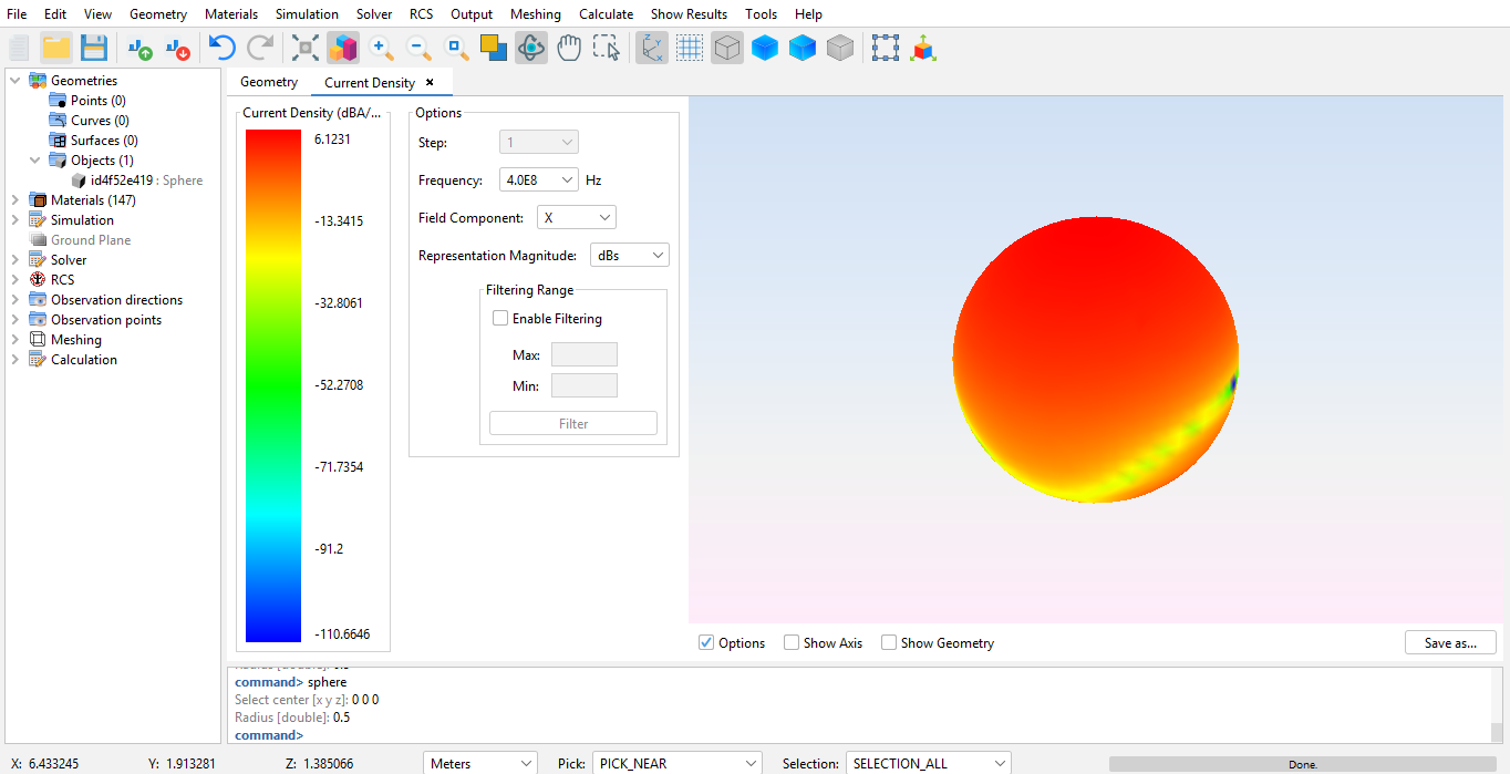
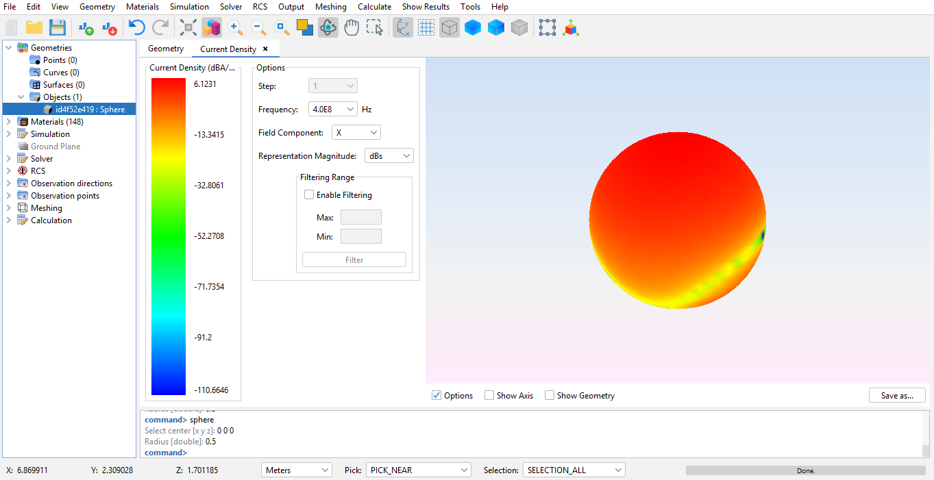
Step 14
Select the Show Results → View Currents option.
Figure 18. Current Density representation
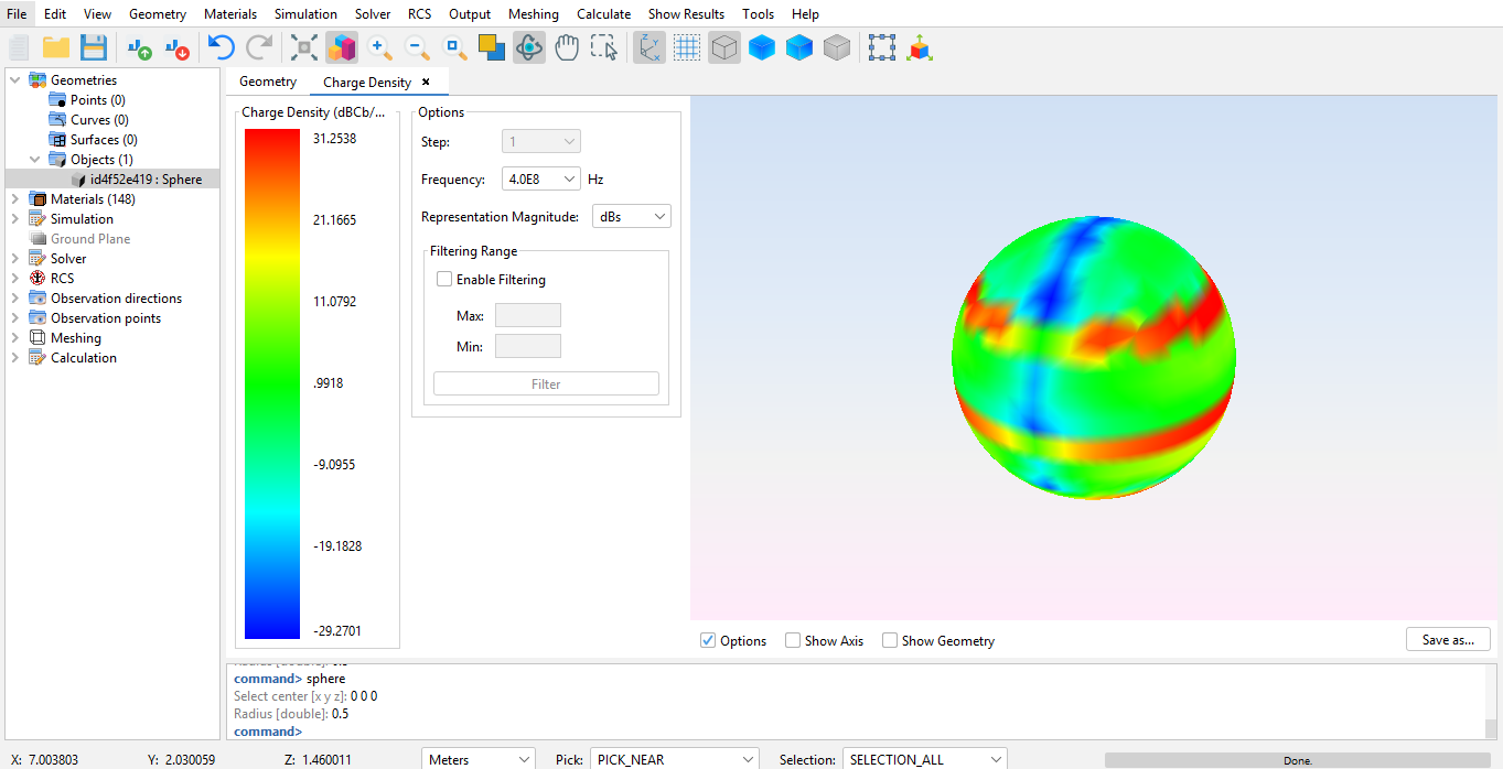
Step 15
Select the Show Results → View Charge option.
Figure 19. Charge Density representation
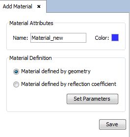
Step 16
Select Materials → Add option.
Figure 20. Add material panel
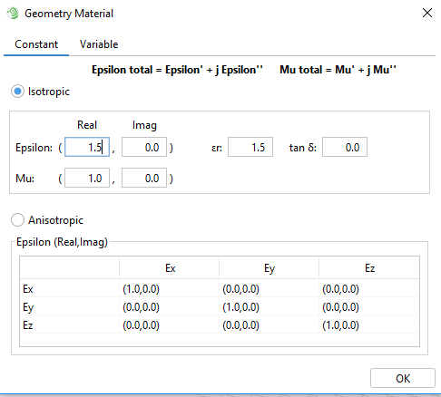
Step 17
Select Material defined by Geometry option and press the Set Parameters button, to
configure as shown the material properties.
Figure 21. Geometry material parameters
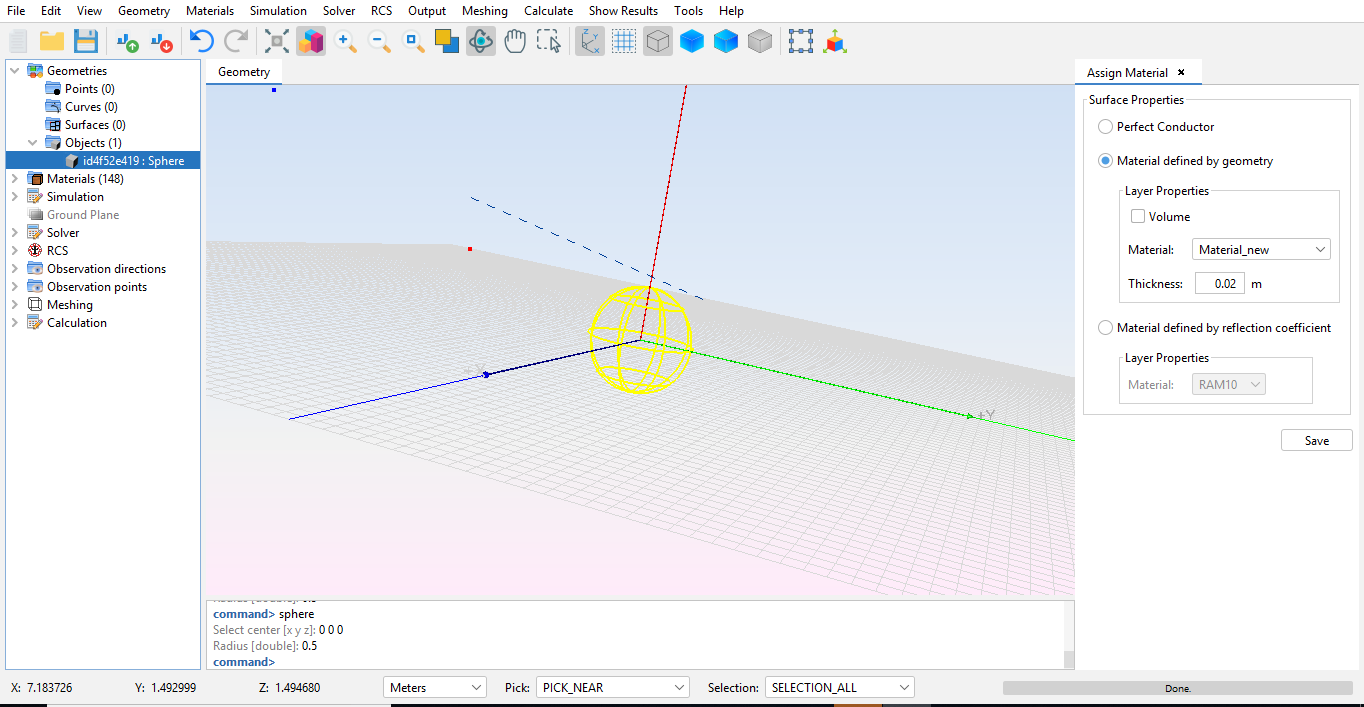
Step 18
Select the geometry on the screen and click on Material → Assign to assign the new
material to those surfaces. Choose the material and specified the thickness.
Figure 22. Geometry selection
Step 19
Mesh the geometry and run the simulation again.
Step 20
Select the option Show Results → Far Field → View Cuts.