Annex 2: Analysis of a Reflectarray Database Creation

This chapter analizes the squared geometry model proposed by F. Zubir et al.¹

Step 0: Open newFASANT software and generate a new PERIODICAL STRUCTURES project selecting the option on the tab that appears when the 'File --> New' option of the menu bar is selected.

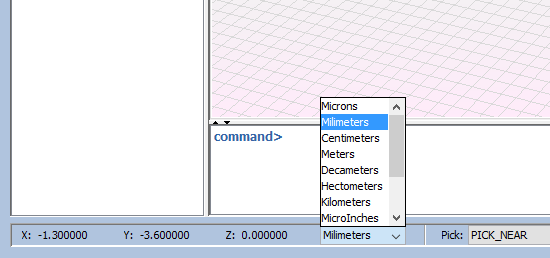
Then, set the interface units on 'millimeters' using the selection list on the bottom left of the main window.

Step 1: Set the variable parameters for the structure. Select "Geometry --> Parameters --> Define Parameters" option on the menu bar. On this tab, all the parameters to be used in the construction of geometry will be set as described in Define Parameters.

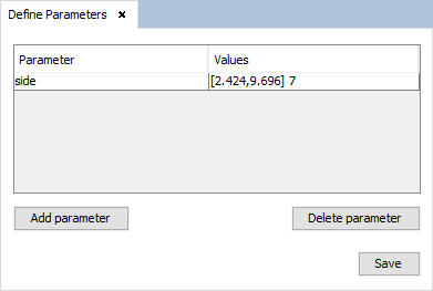
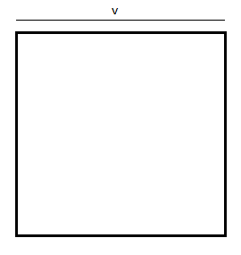
This parameter is referenced to the size of the plane for the resonant frequency at 11 GHz. For this frequency parameter ‘v’ = 6.06mm. This way the plane has 7 different sizes having in the middle step the size of the resonant frequency at 11 GHz and in the upper step the maximum size possible to the cell that will be defined on next steps. Note to use 37 steps for 37 different sizes the parameters must be defined changing the samples value of 7 to 37 on the parameters definition.

Generate a plane typing 'plane' on the command line panel, and introducing the parameters as the next figure shows. To see information about the use of the command line panel, see Command Line.

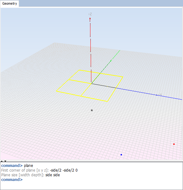
Add a point to add the reference of phase where a ground plane will be placed on the cell definition. Add the point at ‘0, 0, -1.524’. This value is the thickness for the cell layer.

Step 3: Create the material for the layer (see Materials Menu (Periodical Structures Module)). The name used for the new material is RF-35 with the values Epsilon = (3.54, -0.0018) and Mu = (1.0, 0.0).

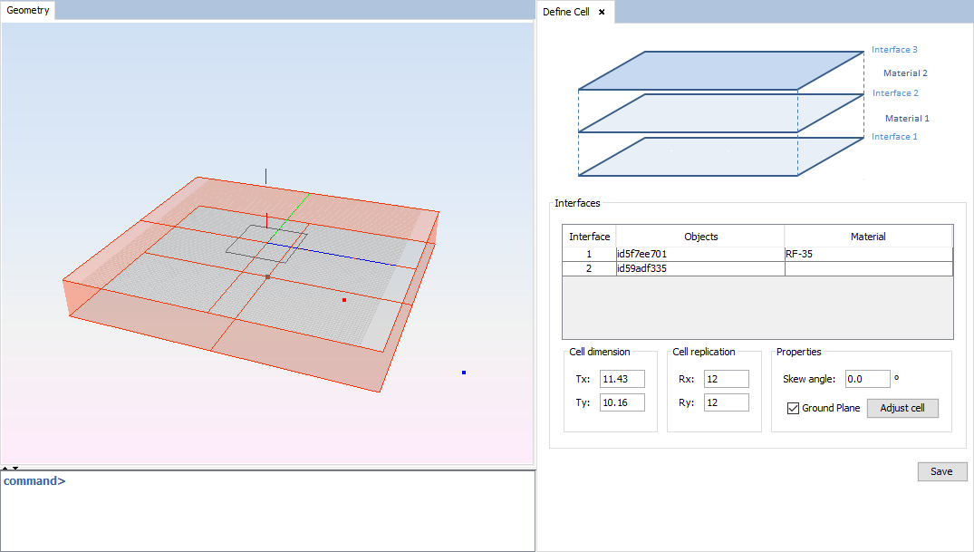
Step 4: Edit the unit cell. Use "Cell --> Define Cell" option for the menu bar. Default, the window takes a size of the cell with the maximum values in X and Y axis, and the first material on the list. Edit the cell as follow:

1. In the table, each row means an interface with it object. The material column refers to the material of the layer above the interface, i.e. the layer between the interface indicate by the row and the next interface. This interfaces are ordered from the lowest Z order to the upper (that can´t has a material). For the material on interface 1 select ‘RF-35’ on the list (the material added on the previous step).
2. For the cell dimension select Tx = 11.43 and Ty = 10.16.
3. For the cell replication, and the skew angle, default values are correct.
4. Set the ground plane, selecting the check box. Then, the floor of the cell will be painted on grey.

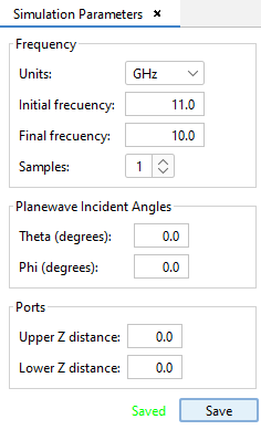
Step 5: Set the simulation parameters using "Simulation --> Parameters" option on the menu bar. This configuration will be identical for both examples.

Set the initial frequency to 11 GHz, the final frequency with default values and the frequency samples set to 1. This options allows to configure a frequency sweep to analyze the cases for different frequencies. For this case only 11 GHz will be analyzed.

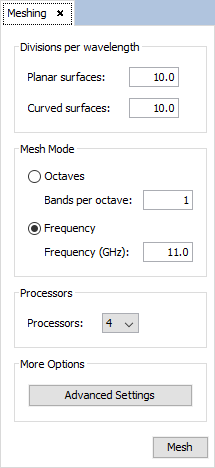
Step 6: Set meshing parameters using "Meshing --> Create Mesh" option on the menu bar.

In this step a meshing with 10 and 20 divisions per wavelength will be compared for the cases with 7 and 37 steps. First, the models will be meshed with 10 divisions per wavelength to the simulation frequency. The number of processors to be selected, to improve the efficiency on time, will be the number of the processors of the machine where the example will be executed.

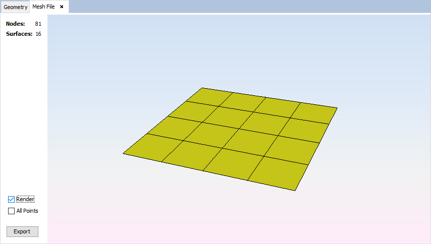
Then, the simulations for each size of the cell component will be executed. When the execution has finished the result meshes can be opened with "Meshing --> Visualize an existing Mesh" option on the menu bar, and selecting the ‘fss_1.msh’ (mesh of the unitary element) file from the directory of the selected step and frequency. The next images corresponds with the files of the last size (‘step6’ or ‘step36’) and the unique frequency (‘f0’). On this steps the difference between 10 and 20 divisions is greater than on ‘step0’ because the size is the biggest on the cases and on the ‘step0’ the size is low to generate differences.

The next image corresponds with the mesh with 10 divisions per wavelength. This result is identical for the cases of 7 and 37 steps.

Then, meshing the structures with 20 divisions per wavelength, the meshes will be larger and the results will be more efficient. The next image corresponds with the mesh with 20 divisions per wavelength. This result is identical for the cases of 7 and 37 steps.

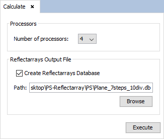
Step 7: Set calculate parameters using "Calculate --> Execute" option on the menu bar. The number of processors to be selected, to improve the efficiency on time, will be the number of the processors of the machine where the example will be executed. Select the path for the database file, previously checked the box to generate it.

Then, the simulations for each size of the cell component will be executed. When the simulations finish the results will be enabled to display it.

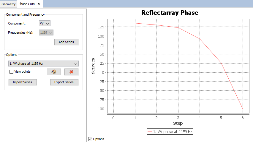
Step 8: Display the information about the phase with "Show Results --> Show Rx/Tx Phase".

First see the phase for the case with 7 steps and 10 divisions per wavelength.

Then see the information for case with 7 steps and 20 divisions.

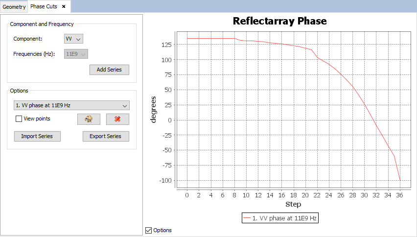
Now see the case with 37 steps and 10 divisions.

Then see the information for case with 37 steps and 20 divisions.

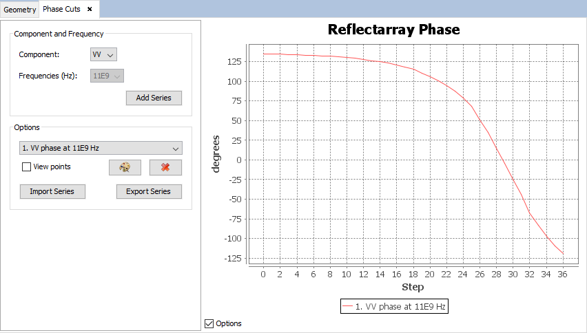
Analyzing the results we can see that on reflectarray cases with elementary cell of size around millimeters is recommended 20 or more divisions per wavelength. On reflectarray cases, to improve the quality of the results is recommended to have a sufficient number of sizes for the unitary cell.