Continuum Analysis
The continuum analysis feature within the EDEM analyst allows users to view and analyze their simulation data as a continuum instead of discrete particles.
Continuum analysis has the benefit of both identifying phenomena that otherwise wouldn’t be obvious and analyzing particle data using continuum based theories. The following continuum quantities can be calculated:
- Granular temperature
- Kinetic pressure
- Mass density
- Momentum density
- Porosity
- Solid fraction
- Velocity
- Shear stress
- Normal stress
Calculation Method
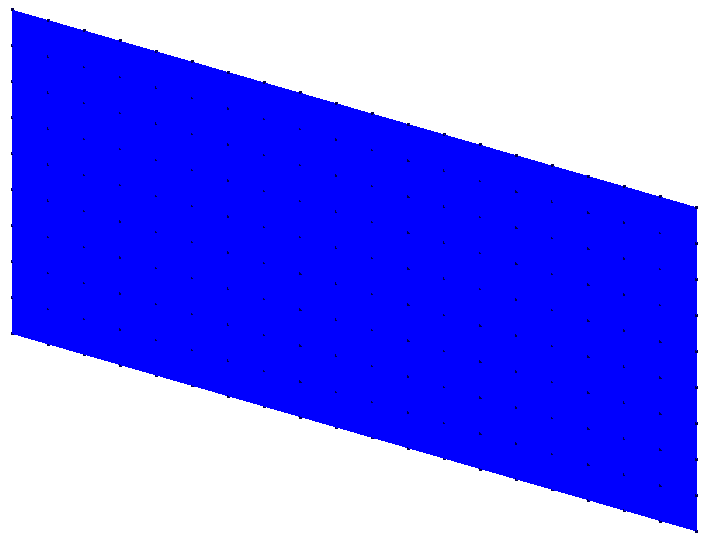
Planes that are made up of evaluation points as seen below are used to create continuum planes that have particle data applied to each evaluation point.
To calculate the continuum values at each evaluation point, a distance weighted sum of the particle data is performed using a Gaussian weighting function seen below. Where Φ(r) is the gaussian distribution function relative to the distance, r, a given particle is away from a given point.

The cut-off distance is used to determine the width of the distribution function used. Using the above equation, 99% of the function's weighting is within a sphere of influence with a radius equal to the cut-off distance. Particles outside the sphere of influence of an evaluation point will not be included in the continuum calculation for that point. This is a parameter that users can change based on their particle data although a value of nine times the average particle diameters is typically recommended, especially if the particle size distribution is narrow.
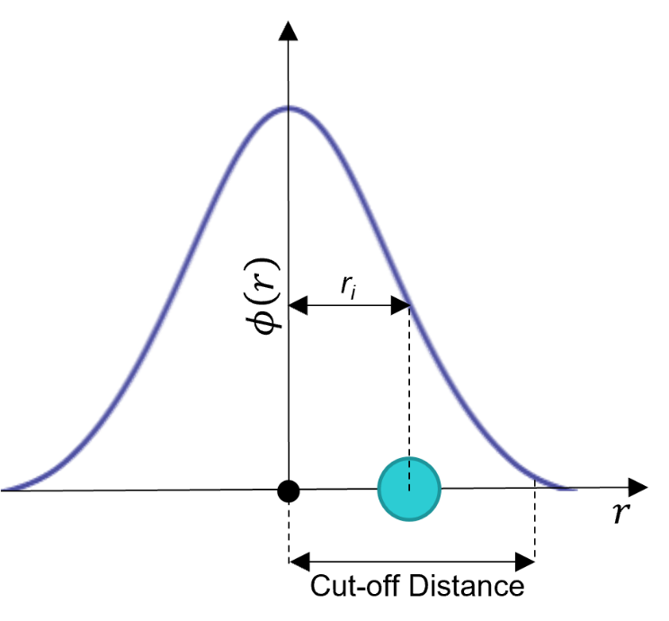
Figure 1 Gaussian Distribution Function
The following are equations used to extract particle data and apply attribute values to the evaluation points using the gaussian distribution function.
Mass density
Where ρ(r,t) is the mass density, is the mass of the particle, and is the gaussian function weighting.

Momentum density
The magnitude of the momentum density can be analyzed along with the X, Y, and Z components.

Granular temperature
Where tg is the granular temperature, vi(t) is velocity and v(ri(t),t) is velocity of particle

Kinetic pressure
Where q is the kinetic pressure, ρ is the mass density, and v is the velocity.

Solid fraction
The solid fraction, Φ,is calculated by dividing the mass density, ρ, by the particle’s solid density, ρs.

Porosity
The porosity is the inverse of the Solid Fraction
Velocity
The velocity, v(r,t), is calculated by dividing the Momentum density by mass density. The magnitude of the velocity can be analyzed along with the X, Y, and Z components.
Shear and Normal Stress
Shear: XY, YZ, and ZX Normal: XX, YY, and ZZ

Creating a Continuum Analysis
Creating a Continuum Item
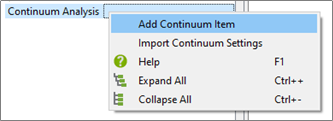
In the Analyst Tree, right-click Continuum Analysis and select Add Continuum Item.
A continuum Item is used to create and define continuum planes, generate data and view the results. The user can add as many planes or plane groups as necessary for each continuum item. Multiple continuum Items can be added or copied.
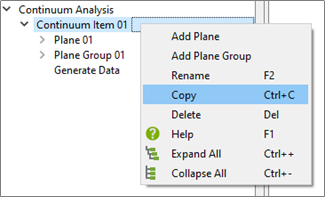
Adding a Plane or Plane Group
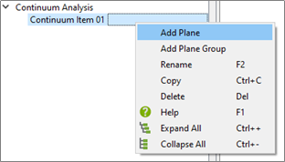
Right-click on Continuum Item and select either Add Plane or Add Plane Group.
Adding a plane will create a single plane in the center of the simulation domain.
Adding a plane group will create a series of planes. The default number of planes and spacing between planes are determined based on the average radius of particles in the simulation with a maximum number created by default of 10.
Modify Plane or Plane Group
The size, position, rotation, and number of evaluation points can be edited for each plane or plane group.
The Display Planes and Display Points tick boxes are used to view the set-up of the analysis planes before data is generated.
The Resize to Domain button can be used to re-set the plane or plane group to its original position, in the XY plane, spanning the domain. Sides A and B’s dimensions can be adjusted to alter the size of the planes manually
The Number of evaluation points can be increased to improve the definition of the continuum data although an increased number of points will increase the data generation time. The number of points can also be defined by using the separation between points.
When defining a plane group, the number of planes and spacing between each plane can be defined within the plane group editor.
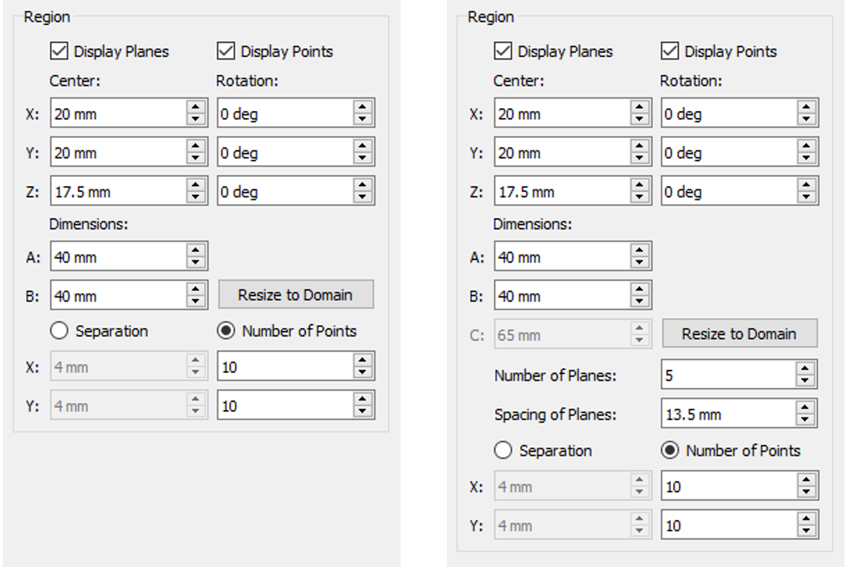
Plane Editor Plane Group Editor
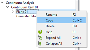
Copy Plane or Plane Group
Planes and Plane Groups can be copied by right-clicking on the plane or plane group and selecting copy. This will copy the plane within the same continuum Item.
Copy Continuum Item
Continuum Items can be copied by right-clicking on the continuum item and selecting copy. This will copy
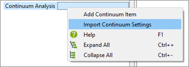
Import Continuum Settings
A continuum Item can be imported from another deck by right-clicking Continuum Analysis and selecting Import Continuum Settings. This will open the file explorer where the user can select an efd file from any deck. If there is a continuum analysis saved in the imported efd file, all continuum settings will be imported but the continuum data associated with the imported continuum items will not be.
Generate Data
After the planes and plane groups are set up, continuum data can be generated. Continuum data cannot be generated on partial time step saves. Three types of analysis can be conducted:
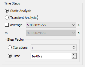
Static Analysis
Static analysis will generate continuum data for a single timestep.
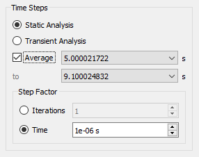
Static Average Analysis
Static average analysis will generate continuum data averaged over a specified range of timesteps.
Transient Analysis
A Transient analysis will generate continuum data for each time step over a specified range of timesteps.
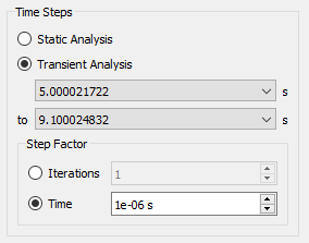
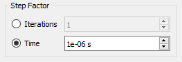
Step Factor
The step factor can be used to step over a set number of time steps when calculating either an averaged or transient analysis.
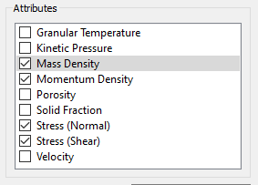
Attributes
The user is required to select each attribute that they want to be generated. Each attribute adds the calculation time of the continuum data so only the required attributes should be selected.
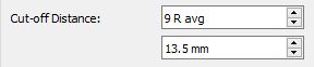
Cut-off Distance
The cut-off distance defines the width of the gaussian weighting function and is equal to the radius of the sphere of influence of the Gaussian function for each evaluation point.
The cut-off distance is automatically 9 times the average particle radius within the simulation. This is recommended for most simulations but testing of different cut-off distances may be required for large size distributions.
Once the data generation settings have been defined, click Generate Data. This will generate the continuum data for all the planes and plane groups contained within the continuum item.
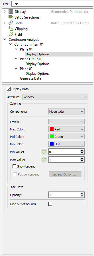
Display Options
To display the continuum data, select either the Display Options within any plane or plane group to edit the settings of those individual planes or plane groups.
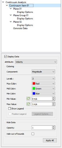
To apply display settings to all planes and plane groups within a continuum item, select the continuum item as seen below. Display settings can then be applied to all planes with the Apply all button at the bottom of the settings window.
[1] Goldhirsch, I. (2010). Stress, stress asymmetry and coupled stress: From discrete particles to continuous fields. Granular Matter, 12(3), 239–252.