Package Modelica.​Fluid.​Utilities
Utility models to construct fluid components (should not be used directly)

Information

Extends from Modelica.​Icons.​UtilitiesPackage (Icon for utility packages).

Package Contents

Function Modelica.​Fluid.​Utilities.​checkBoundary
Check whether boundary definition is correct

Information

This icon indicates Modelica functions.

Extends from Modelica.​Icons.​Function (Icon for functions).

Inputs

Function Modelica.​Fluid.​Utilities.​regRoot
Anti-symmetric square root approximation with finite derivative in the origin

Information

This function approximates sqrt(abs(x))*sgn(x), such that the derivative is finite and smooth in x=0.

With the default value of delta=0.01, the difference between sqrt(x) and regRoot(x) is 16% around x=0.01, 0.25% around x=0.1 and 0.0025% around x=1.

Extends from Modelica.​Icons.​Function (Icon for functions).

Inputs

Outputs

Function Modelica.​Fluid.​Utilities.​regRoot_der
Derivative of regRoot

Information

Extends from Modelica.​Icons.​Function (Icon for functions).

Inputs

Outputs

Function Modelica.​Fluid.​Utilities.​regSquare
Anti-symmetric square approximation with non-zero derivative in the origin

Information

This function approximates x^2*sgn(x), such that the derivative is non-zero in x=0.

With the default value of delta=0.01, the difference between x^2 and regSquare(x) is 41% around x=0.01, 0.4% around x=0.1 and 0.005% around x=1.

Extends from Modelica.​Icons.​Function (Icon for functions).

Inputs

Outputs

Function Modelica.​Fluid.​Utilities.​regPow
Anti-symmetric power approximation with non-zero derivative in the origin

Information

This function approximates abs(x)^a*sign(x), such that the derivative is positive, finite and smooth in x=0.

Extends from Modelica.​Icons.​Function (Icon for functions).

Inputs

Outputs

Function Modelica.​Fluid.​Utilities.​regRoot2
Anti-symmetric approximation of square root with discontinuous factor so that the first derivative is finite and continuous

Information

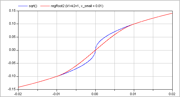
Approximates the function

   y = if x ≥ 0 then sqrt(k1*x) else -sqrt(k2*abs(x)), with k1, k2 ≥ 0

in such a way that within the region -x_small ≤ x ≤ x_small, the function is described by two polynomials of third order (one in the region -x_small .. 0 and one within the region 0 .. x_small) such that

• The derivative at x=0 is finite.
• The overall function is continuous with a continuous first derivative everywhere.
• If parameter use_yd0 = false, the two polynomials are constructed such that the second derivatives at x=0 are identical. If use_yd0 = true, the derivative at x=0 is explicitly provided via the additional argument yd0. If necessary, the derivative yd0 is automatically reduced in order that the polynomials are strict monotonically increasing [Fritsch and Carlson, 1980].

Typical screenshots for two different configurations are shown below. The first one with k1=k2=1:

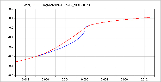
and the second one with k1=1 and k2=3:

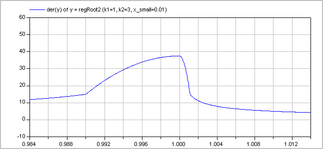
The (smooth) derivative of the function with k1=1, k2=3 is shown in the next figure:

Literature

Fritsch F.N. and Carlson R.E. (1980):

Monotone piecewise cubic interpolation. SIAM J. Numerc. Anal., Vol. 17, No. 2, April 1980, pp. 238-246

Extends from Modelica.​Icons.​Function (Icon for functions).

Inputs

Outputs

Function Modelica.​Fluid.​Utilities.​regSquare2
Anti-symmetric approximation of square with discontinuous factor so that the first derivative is non-zero and is continuous

Information

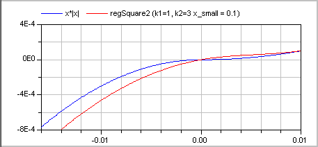
Approximates the function

   y = if x ≥ 0 then k1*x*x else -k2*x*x, with k1, k2 > 0

in such a way that within the region -x_small ≤ x ≤ x_small, the function is described by two polynomials of third order (one in the region -x_small .. 0 and one within the region 0 .. x_small) such that

• The derivative at x=0 is non-zero (in order that the inverse of the function does not have an infinite derivative).
• The overall function is continuous with a continuous first derivative everywhere.
• If parameter use_yd0 = false, the two polynomials are constructed such that the second derivatives at x=0 are identical. If use_yd0 = true, the derivative at x=0 is explicitly provided via the additional argument yd0. If necessary, the derivative yd0 is automatically reduced in order that the polynomials are strict monotonically increasing [Fritsch and Carlson, 1980].

A typical screenshot for k1=1, k2=3 is shown in the next figure:

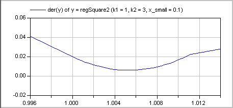
The (smooth, non-zero) derivative of the function with k1=1, k2=3 is shown in the next figure:

Literature

Fritsch F.N. and Carlson R.E. (1980):

Monotone piecewise cubic interpolation. SIAM J. Numerc. Anal., Vol. 17, No. 2, April 1980, pp. 238-246

Extends from Modelica.​Icons.​Function (Icon for functions).

Inputs

Outputs

Function Modelica.​Fluid.​Utilities.​regStep
Approximation of a general step, such that the characteristic is continuous and differentiable

Information

This function is used to approximate the equation

    y = if x > 0 then y1 else y2;

by a smooth characteristic, so that the expression is continuous and differentiable:

   y = smooth(1, if x >  x_small then y1 else
                 if x < -x_small then y2 else f(y1, y2));

In the region -x_small < x < x_small a 2nd order polynomial is used for a smooth transition from y1 to y2.

Extends from Modelica.​Icons.​Function (Icon for functions).

Inputs

Outputs

Function Modelica.​Fluid.​Utilities.​evaluatePoly3_derivativeAtZero
Evaluate polynomial of order 3 that passes the origin with a predefined derivative

Information

Extends from Modelica.​Icons.​Function (Icon for functions).

Inputs

Outputs

Function Modelica.​Fluid.​Utilities.​regFun3
Co-monotonic and C1 smooth regularization function

Information

Approximates a function in a region between x0 and x1 such that

• The overall function is continuous with a continuous first derivative everywhere.
• The function is co-monotone with the given data points.

In this region, a continuation is constructed from the given points (x0, y0), (x1, y1) and the respective derivatives. For this purpose, a single polynomial of third order or two cubic polynomials with a linear section in between are used [Gasparo and Morandi, 1991]. This algorithm was extended with two additional conditions to avoid saddle points with zero/infinite derivative that lead to integrator step size reduction to zero.

This function was developed for pressure loss correlations properly addressing the static head on top of the established requirements for monotonicity and smoothness. In this case, the present function allows to implement the exact solution in the limit of x1-x0 -> 0 or y1-y0 -> 0.

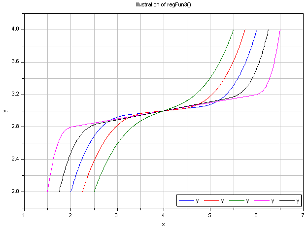
Typical screenshots for two different configurations are shown below. The first one illustrates five different settings of xi and yid:

The second graph shows the continuous derivative of this regularization function:

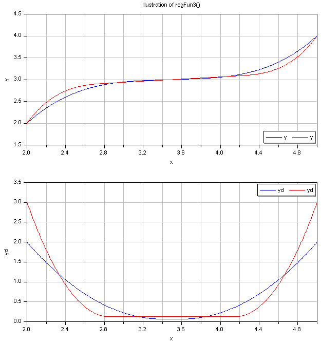
Literature

Gasparo M. G. and Morandi R. (1991):

Piecewise cubic monotone interpolation with assigned slopes. Computing, Vol. 46, Issue 4, December 1991, pp. 355 - 365.

Extends from Modelica.​Icons.​Function (Icon for functions).

Inputs

Outputs

Function Modelica.​Fluid.​Utilities.​cubicHermite
Evaluate a cubic Hermite spline

Information

This icon indicates Modelica functions.

Extends from Modelica.​Icons.​Function (Icon for functions).

Inputs

Outputs

Function Modelica.​Fluid.​Utilities.​cubicHermite_withDerivative
Evaluate a cubic Hermite spline, return value and derivative

Information

This icon indicates Modelica functions.

Extends from Modelica.​Icons.​Function (Icon for functions).

Inputs

Outputs