 Package Modelica.Mechanics.Translational.Examples
Demonstration examples of the components of this package
Package Modelica.Mechanics.Translational.Examples
This package contains example models to demonstrate the usage of the Translational package. Open the models and simulate them according to the provided description in the models.
Extends from Modelica.Icons.ExamplesPackage (Icon for packages containing runnable examples).
| Name | Description |
|---|---|
Accelerate | Use of model accelerate |
Brake | Demonstrate braking of a translational moving mass |
Damper | Use of damper models |
EddyCurrentBrake | Demonstrate the usage of the translational eddy current brake |
ElastoGap | Demonstrate usage of ElastoGap |
Friction | Use of model Stop |
GenerationOfFMUs | Example to demonstrate variants to generate FMUs (Functional Mock-up Units) |
HeatLosses | Demonstrate the modeling of heat losses |
InitialConditions | Setting of initial conditions |
Oscillator | Oscillator demonstrates the use of initial conditions |
PreLoad | Preload of a spool using ElastoGap models |
Sensors | Sensors for translational systems |
SignConvention | Examples for the used sign conventions |
Utilities … | Utility classes used by translational example models |
WhyArrows | Use of arrows in Mechanics.Translational |
 Model Modelica.Mechanics.Translational.Examples.SignConvention
If all arrows point in the same direction, a positive force results in a positive acceleration a, velocity v and position s.
For a force of 1 N and a mass of 1 kg this leads to
a = 1 m/s2
v = 1 m/s after 1 s (SlidingMass1.v)
s = 0.5 m after 1 s (SlidingMass1.s)
The acceleration is not available for plotting.
System 1) and 2) are equivalent. It doesn't matter whether the force pushes at flange_a in system 1 or pulls at flange_b in system 2.
It is of course possible to ignore the arrows and connect the models in an arbitrary way. But then it is hard see in what direction the force acts.
In the third system the two arrows are opposed which means that the force acts in the opposite direction (in the same direction as in the two other examples).
Extends from Modelica.Icons.Example (Icon for runnable examples).
 Model Modelica.Mechanics.Translational.Examples.InitialConditions
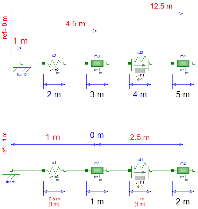
There are several ways to set initial conditions. In the first system the position of the mass m3 was defined by using the modifier s(start=4.5), the position of m4 by s(start=12.5). These positions were chosen such that the system is at rest. To calculate these values start at the left (fixed2) with a value of 1 m. The spring s2 has an unstretched length of 2 m and m3 an length of 3 m, which leads to
  1   m (fixed2)
+ 2   m (spring s2)
+ 3/2 m (half of the length of mass m3)
-------
  4,5 m = s(start = 4.5) for m3
+ 3/2 m (half of the length of mass m3)
+ 4   m (springDamper sd2)
+ 5/2 m (half of length of mass m4)
-------
 12,5 m = s(start = 12.5) for m4
This selection of initial conditions can prioritize the selection of those variables (m3.s and m4.s) as state variables.
In the second example, the lengths of the springs are given start values but they cannot be used as state for pure springs (only for the spring/damper combination). In this case the system is not at rest.
Extends from Modelica.Icons.Example (Icon for runnable examples).
 Model Modelica.Mechanics.Translational.Examples.WhyArrows
When using the models of the translational sublibrary it is recommended to make sure that all arrows point in the same direction because then all component have the same reference system. In the example the distance from flange_a of Rod1 to flange_b of Rod2 is 2 m. The distance from flange_a of Rod1 to flange_b of Rod3 is also 2 m though it is difficult to see that. Without the arrows it would be almost impossible to notice. That all arrows point in the same direction is a sufficient condition for an easy use of the library. There are cases where horizontally flipped models can be used without problems.
Extends from Modelica.Icons.Example (Icon for runnable examples).
 Model Modelica.Mechanics.Translational.Examples.Accelerate
Demonstrate usage of component Sources.Accelerate by moving a mass with a predefined acceleration.
Extends from Modelica.Icons.Example (Icon for runnable examples).
 Model Modelica.Mechanics.Translational.Examples.Damper
Demonstrate usage of a translational damper component in various configurations.
Extends from Modelica.Icons.Example (Icon for runnable examples).
 Model Modelica.Mechanics.Translational.Examples.Oscillator
A spring - mass system is a mechanical oscillator. If no damping is included and the system is excited at resonance frequency infinite amplitudes will result. The resonant frequency is given by omega_res = sqrt(c / m) with:
c ... spring stiffness
m ... mass
To make sure that the system is initially at rest the initial conditions s(start=-0.5) and v(start=0) for the sliding masses are set. If damping is added the amplitudes are bounded.
Extends from Modelica.Icons.Example (Icon for runnable examples).
 Model Modelica.Mechanics.Translational.Examples.Sensors
These sensors measure
force f in N
position s in m
velocity v in m/s
acceleration a in m/s2
In this example, the measured velocity and acceleration is independent of
the flange the sensor is connected to. In contrast, the measured position
depends on the flange (flange_a or flange_b) and the
length L of the component.
Plot positionSensor1.s, positionSensor2.s and mass.s
to see the difference.
Extends from Modelica.Icons.Example (Icon for runnable examples).
 Model Modelica.Mechanics.Translational.Examples.Friction
Extends from Modelica.Icons.Example (Icon for runnable examples).
 Model Modelica.Mechanics.Translational.Examples.PreLoad
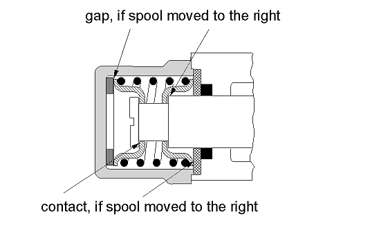
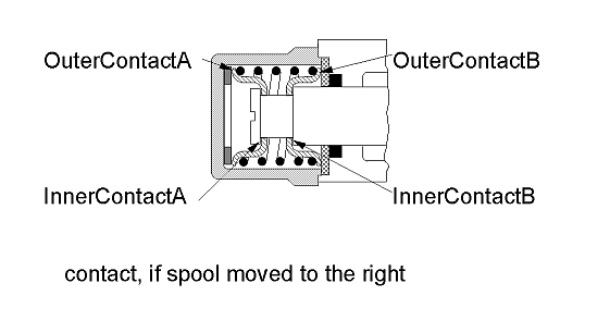
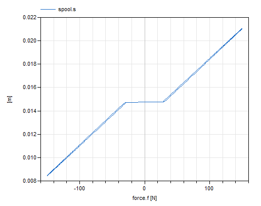
When designing hydraulic valves it is often necessary to hold the spool in a certain position as long as an external force is below a threshold value. If this force exceeds the threshold value a linear relation between force and position is desired. There are designs that need only one spring to accomplish this task. Using the ElastoGap elements this design can be modelled easily. Drawing of spool.
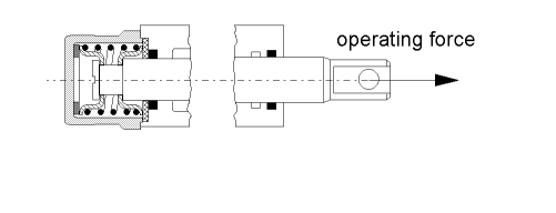
Simulate for 100 s and plot the spool position spool.s
as a function of working force force.f.
For positive force, the spool moves in positive direction - in figure below
the start value spool.s.start influences the offset.
.
Extends from Modelica.Icons.Example (Icon for runnable examples).
 Model Modelica.Mechanics.Translational.Examples.ElastoGap
This model demonstrates the effect of ElastoGaps on eigenfrequency: Plot mass1.s and mass2.s as well as mass1.v and mass2.v to see that effect.
While mass1 is moved by both spring/damper forces all the time, this is not the case for mass2 since elastoGap1 lifts off at s > -0.5 m and elastoGap2 lifts off at s < +0.5 m. Therefore, mass2 moves freely as long as -0.5 m < s < +0.5 m.
Extends from Modelica.Icons.Example (Icon for runnable examples).
| Type | Name | Default | Description |
|---|---|---|---|
TranslationalDampingConstant | d | 1.5 | Damping constant |
 Model Modelica.Mechanics.Translational.Examples.Brake
This model consists of a mass with an initial velocity of 1 m/s. After 0.1 s, a brake is activated and it is shown that the mass decelerates until it arrives at rest and remains at rest. Two versions of this system are present, one where the brake is implicitly grounded and one where it is grounded explicitly.
Extends from Modelica.Icons.Example (Icon for runnable examples).
 Model Modelica.Mechanics.Translational.Examples.HeatLosses
This model demonstrates how to model the dissipated power of a Translational model, by enabling the heatPort of all components and connecting these heatPorts via a convection element to the environment. The total heat flow generated by the elements and transported to the environment is present in variable convection.fluid.
Extends from Modelica.Icons.Example (Icon for runnable examples).
 Model Modelica.Mechanics.Translational.Examples.EddyCurrentBrake
An eddy current brake reduces the speed of a moving mass. Kinetic energy is converted to thermal energy which leads to a temperature increase of the thermal capacitance of the brake, which can be assumed as adiabatic during the rather short time span of the braking.
Extends from Modelica.Icons.Example (Icon for runnable examples).
 Model Modelica.Mechanics.Translational.Examples.GenerationOfFMUs
This example demonstrates how to generate an input/output block (e.g. in form of an FMU - Functional Mock-up Unit) from various Translational components. The goal is to export such an input/output block from Modelica and import it in another modeling environment. The essential issue is that before exporting it must be known in which way the component is utilized in the target environment. Depending on the target usage, different flange variables need to be in the interface with either input or output causality. Note, this example model can be used to test the FMU export/import of a Modelica tool. Just export the components marked in the icons as "toFMU" as FMUs and import them back. The models should then still work and give the same results as a pure Modelica model.
Connecting two masses
The upper part (DirectMass, InverseMass)
demonstrates how to export two masses and connect them
together in a target system. This requires that one of the masses
(here: DirectMass)
is defined to have states and the position, velocity and
acceleration are provided in the interface.
The other mass (here: InverseMass) is moved according
to the provided input position, velocity and acceleration.
Connecting a force element that needs position and velocities
The middle part (SpringDamper) demonstrates how to export a force element
that needs both position and velocities for its force law and connect this
force law in a target system between two masses.
Connecting a force element that needs only positions
The lower part (Spring) demonstrates how to export a force element
that needs only positions for its force law and connect this
force law in a target system between two masses.
Extends from Modelica.Icons.Example (Icon for runnable examples).