Package Modelica.​StateGraph.​UsersGuide
User's Guide of StateGraph Library

Information

Library StateGraph is a free Modelica package providing components to model discrete event and reactive systems in a convenient way. This package contains the User's Guide for the library and has the following content:

1. Overview of library gives an overview of the library.
2. A first example demonstrates at hand of a first example how to use this library.
3. An application example demonstrates varies features at hand of the control of a two tank system.
4. Comparison with StateGraph2 compares Modelica.StateGraph with the much improved version Modelica_StateGraph2.
5. Release Notes summarizes the differences between different versions of this library.
6. Literature provides references that have been used to design and implement this library.
7. Contact provides information about the authors of the library as well as acknowledgments.

Extends from Modelica.​Icons.​Information (Icon for general information packages).

Package Contents

Class Modelica.​StateGraph.​UsersGuide.​OverView
Overview of library

Information

In this section, an overview of the most important features of this library is given.

Steps and Transitions

A StateGraph is an enhanced finite state machine. It is based on the JGrafchart method and takes advantage of Modelica features for the "action" language. JGrafchart is a further development of Grafcet to include elements of StateCharts that are not present in Grafcet/Sequential Function Charts. Therefore, the StateGraph library has a similar modeling power as StateCharts but avoids some deficiencies of StateCharts.

The basic elements of StateGraphs are steps and transitions:

Steps represent the possible states a StateGraph can have. If a step is active the Boolean variable active of the step is true. If it is deactivated, active = false. At the initial time, all "usual" steps are deactivated. The InitialStep objects are steps that are activated at the initial time. They are characterized by a double box (see figure above).

Transitions are used to change the state of a StateGraph. When the step connected to the input of a transition is active, the step connected to the output of this transition is deactivated and the transition condition becomes true, then the transition fires. This means that the step connected to the input to the transition is deactivated and the step connected to the output of the transition is activated.

The transition condition is defined via the parameter menu of the transition object. Clicking on object "transition1" in the above figure, results in the following menu:

In the input field "condition", any type of time varying Boolean expression can be given (in Modelica notation, this is a modification of the time varying variable condition). Whenever this condition is true, the transition can fire. Additionally, it is possible to activate a timer, via enableTimer (see menu above) and provide a waitTime. In this case the firing of the transition is delayed according to the provided waitTime. The transition condition and the waitTime are displayed in the transition icon.

In the above example, the simulation starts at initialStep. After 1 second, transition1 fires and step1 becomes active. After another second transition2 fires and initialStep becomes again active. After a further second step1 becomes again active, and so on.

In JGrafcharts, Grafcet and Sequential Function Charts, the network of steps and transitions is drawn from top to bottom. In StateGraphs, no particular direction is defined, since steps and transitions are blocks with input and output connectors that can be arbitrarily placed and connected. Usually, it is most practical to define the network from left to right, as in the example above, since then it is easy to read the labels on the icons.

Conditions and Actions

With the block TransitionWithSignal, the firing condition can be provided as Boolean input signal, instead as entry in the menu of the transition. An example is given in the next figure:

Component "step" is an instance of "StepWithSignal" that is a usual step where the active flag is available as Boolean output signal. To this output, component "Timer" from library "Modelica.Blocks.Logical" is connected. It measures the time from the time instant where the Boolean input (i.e., the active flag of the step) became true up to the current time instant. The timer is connected to a comparison component. The output is true, once the timer reaches 1 second. This signal is used as condition input of the transition. As a result, "transition2" fires, once step "step" has been active for 1 second. Of course, any other Modelica block with a Boolean output signal can be connected to the condition input of such a transition block as well.

Conditions of a transition can either be computed by a network of logical blocks from the Logical library as in the figure above, or via the "SetBoolean" component any type of logical expression can be defined in textual form, as shown in the next figure:

With the block "SetBoolean", a time varying expression can be provided as modification to the output signal y (see block with icon text "timer.y > 1" in the figure above). The output signal can be in turn connected to the condition input of a TransitionWithSignal block.

The "SetBoolean" block can also be used to compute a Boolean signal depending on the active step. In the figure above, the output of the block with the icon text "step.active" is true, when "step" is active, otherwise it is false (note, the icon text of "SetBoolean" displays the modification of the output signal "y"). This signal can then be used to compute desired actions in the physical systems model. For example, if a valve shall be open, when the StateGraph is in "step1" or in "step4", a "SetBoolean" block may be connected to the valve model using the following condition:

    valve = step1.active or step2.active

Via the Modelica operators edge(..) and change(..), conditions depending on rising and falling edges of Boolean expressions can be used when needed.

In JGrafcharts, Grafcet, Sequential Function Charts and StateCharts, actions are formulated within a step. Such actions are distinguished as entry, normal, exit and abort actions. For example, a valve might be opened by an entry action of a step and might be closed by an exit action of the same step. In StateGraphs, this is (fortunately) not possible due to Modelica's "single assignment rule" that requires that every variable is defined by exactly one equation. Instead, the approach explained above is used. For example, via the "SetBoolean" component, the valve variable is set to true when the StateGraph is in particular steps.

This feature of a StateGraph is very useful, since it allows a Modelica translator to guarantee that a given StateGraph has always deterministic behaviour without conflicts. In the other methodologies this is much more cumbersome. For example, if two steps are executed in parallel and both step actions modify the same variable, the result is either non-deterministic or non-obvious rules have to be defined which action takes priority. In a StateGraph, such a situation is detected by the translator resulting in an error, since there are two equations to compute one variable. Additional benefits of the StateGraph approach are:

• A JGrafchart or a StateChart need to potentially access variables in a step that are defined in higher hierarchical levels of a model. Therefore, mostly global variables are used in the whole network, even if the network is structured hierarchically. In StateGraphs this is not necessary, since the physical systems outside of a StateGraph might access the step or transition state via a hierarchical name. This means that no global variables are needed, because the local variables in the StateGraph are accessed from local variables outside of the StateGraph.
• It is simpler for a user to understand the information that is provided in the non-graphical definition, since every variable is defined at exactly one place. In the other methodologies, the setting and re-setting of the same variable is cluttered within the whole network.

To emphasize this important difference between these methodologies, consider the case that a state machine has the following hierarchy:

   stateMachine.superstate1.superstate2.step1

Within "step1" a StateChart would, e.g., access variable "stateMachine.openValve", say as "entry action: openValve = true". This typical usage has the severe drawback that it is not possible to use the hierarchical state "superstate1" as component in another context, because "step1" references a particular name outside of this component.

In a StateGraph, there would be typically a "SetBoolean" component in the "stateMachine" component stating:

    openValve = superstate1.superstate2.step1.active;

As a result, the "superstate1" component can be used in another context, because it does not depend on the environment where it is used.

Execution Model

The execution model of a StateGraph follows from its Modelica implementation: Given the states of all steps, i.e., whether a step is active or not active, the equations of all steps, transitions, transition conditions, actions etc. are sorted resulting in an execution sequence to compute essentially the new values of the steps. If conflicts occur, e.g., if there are more equations as variables, of if there are algebraic loops between Boolean variables, an exception is raised. Once all equations have been processed, the active variable of all steps are updated to the newly calculated values. Afterwards, the equations are again evaluated. The iteration stops, once no step changes its state anymore, i.e., once no transition fires anymore. Then, simulation continuous until a new event is triggered, (when a relation changes its value).

With the Modelica "sampled(..)" operator, a StateGraph might also be executed within a discrete controller that is called at regular time instants. In a future version of the StateGraph library, this might be more directly supported.

Parallel and Alternative Execution

Parallel activities can be defined by component Parallel and alternative activities can be defined by component Alternative. An example for both components is given in the next figure.

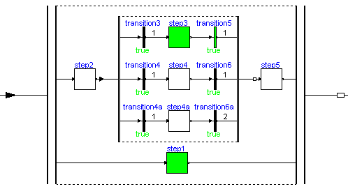
Here, the branch from "step2" to "step5" is executed in parallel to "step1". A transition connected to the output of a parallel branch component can only fire if the final steps in all parallel branches are active simultaneously. The figure above is a screen-shot from the animation of the StateGraph: Whenever a step is active or a transition can fire, the corresponding component is marked in green color.

The three branches within "step2" to "step5" are executed alternatively, depending which transition condition of "transition3", "transition4", "transition4a" fires first. Since all three transitions fire after 1 second, they are all candidates for the active branch. If two or more transitions would fire at the same time instant, a priority selection is made: The alternative and parallel components have a vector of connectors. Every branch has to be connected to exactly one entry of the connector vector. The entry with the lowest number has the highest priority.

Parallel, Alternative and Step components have vectors of connectors. The dimensions of these vectors are set in the corresponding parameter menu. E.g. in a "Parallel" component:

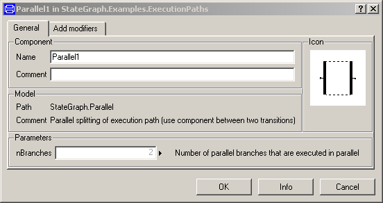
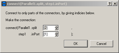
Currently in Dymola the following menu pops up, when a branch is connected to a vector of components in order to define the vector index to which the component shall be connected:

CompositeSteps, Suspend and Resume Port

A StateGraph can be hierarchically structured by using a CompositeStep. This is a component that inherits from PartialCompositeStep. An example is given in the next figure (from Examples.ControlledTanks):

The CompositeStep component contains a local StateGraph that is entered by one or more input transitions and that is left by one or more output transitions. Also, other needed signals may enter a CompositeStep. The CompositeStep has similar properties as a "usual" step: The CompositeStep is active once at least one step within the CompositeStep is active. Variable active defines the state of the CompositeStep.

Additionally, a CompositeStep has a suspend port. Whenever the transition connected to this port fires, the CompositeStep is left at once. When leaving the CompositeStep via the suspend port, the internal state of the CompositeStep is saved, i.e., the active flags of all steps within the CompositeStep. The CompositeStep might be entered via its resume port. In this case the internal state from the suspend transition is reconstructed and the CompositeStep continues the execution that it had before the suspend transition fired (this corresponds to the history ports of StateCharts or JGrafcharts).

A CompositeStep may contain other CompositeSteps. At every level, a CompositeStep and all of its content can be left via its suspend ports (actually, there is a vector of suspend connectors, i.e., a CompositeStep might be aborted due to different transitions).

Extends from Modelica.​Icons.​Information (Icon for general information packages).

Class Modelica.​StateGraph.​UsersGuide.​FirstExample
A first example

Information

A first example will be given here (not yet done).

Extends from Modelica.​Icons.​Information (Icon for general information packages).

Class Modelica.​StateGraph.​UsersGuide.​ApplicationExample
An application example

Information

In this section a more realistic, still simple, application example is given, to demonstrate various features of the StateGraph library. This example shows the control of a two tank system from the master thesis of Isolde Dressler (see literature).

In the following figure the top level of the model is shown. This model is available as StateGraph.Examples.ControlledTanks.

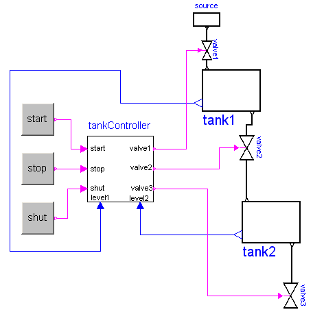
In the right part of the figure, two tanks are shown. At the top part, a large fluid source is present from which fluid can be filled in tank1 when valve1 is open. Tank1 can be emptied via valve2 that is located in the bottom of tank2 and fills a second tank2 which in turn is emptied via valve3. The actual levels of the tanks are measured and are provided as signals level1 and level2 to the tankController.

The tankController is controlled by three buttons, start, stop and shut (for shutdown) that are mutually exclusive. This means that whenever one button is pressed (i.e., its state is true) then the other two buttons are not pressed (i.e., their states are false). When button start is pressed, the "normal" operation to fill and to empty the two tanks is processed:

1. Valve 1 is opened and tank 1 is filled.
2. When tank 1 reaches its fill level limit, valve 1 is closed.
3. After a waiting time, valve 2 is opened and the fluid flows from tank 1 into tank 2.
4. When tank 1 is empty, valve 2 is closed.
5. After a waiting time, valve 3 is opened and the fluid flows out of tank 2
6. When tank 2 is empty, valve 3 is closed

The above "normal" process can be influenced by the following buttons:

• Button start starts the above process. When this button is pressed after a "stop" or "shut" operation, the process operation continues.
• Button stop stops the above process by closing all valves. Then, the controller waits for further input (either "start" or "shut" operation).
• Button shut is used to shutdown the process, by emptying at once both tanks. When this is achieved, the process goes back to its start configuration. Clicking on "start", restarts the process.

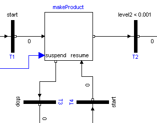
The implementation of the tankController is shown in the next figure:

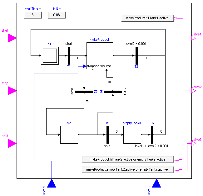
When the "start" button is pressed, the stateGraph is within the CompositeStep "makeProduct". During normal operation this CompositeStep is only left, once tank2 is empty. Afterwards, the CompositeStep is at once re-entered.

When the "stop" button is pressed, the "makeProduct" CompositeStep is at once terminated via the "suspend" port and the stateGraph waits in step "s2" for further commands. When the "start" button is pressed, the CompositeStep is re-entered via its resume port and the "normal" operation continues at the state where it was aborted by the suspend transition. If the "shut" button is pressed, the stateGraph waits in the "emptyTanks" step, until both tanks are empty and then waits at the initial step "s1" for further input.

The opening and closing of valves is not directly defined in the stateGraph. Instead via the "setValveX" components, the Boolean state of the valves are computed. For example, the output y of "setValve2" is computed as:

  y = makeProduct.fillTank2.active or emptyTanks.active

i.e., valve2 is open, when step "makeProduct.fillTank2 or when step "emptyTanks" is active. Otherwise, valve2 is closed.

Extends from Modelica.​Icons.​Information (Icon for general information packages).

Class Modelica.​StateGraph.​UsersGuide.​ComparisonWithStateGraph2
Comparison with StateGraph2

Information

There is a much improved library available called "Modelica_StateGraph2". If this library is not yet distributed with your Modelica tool, you can download it from https://github.com/modelica/Modelica_StateGraph2. Find below a comparison with respect to Modelica.StateGraph. It is not yet clear whether Modelica_StateGraph2 will be included in a future version of the Modelica package. Another option is to provide built-in support for state machines in a future Modelica language version which would allow an even more powerful treatment of state machines in Modelica.

The Modelica_StateGraph2 library (called StateGraph2 below) is based on the experience with the current Modelica.StateGraph library (called StateGraph1 below) and is a significantly further development of StateGraph1. Furthermore, it is heavily based on the article (Malmheden et. al. 2008), see Literature below, but uses a different implementation technique as described in this article. The StateGraph2 library has the following improvements with respect to the StateGraph1 library:

• 3 Basic Components (Step, Transition, Parallel)
  All multiple versions of a component are combined in only one version (e.g., one step and not 4 step components). This is easier to understand and more convenient to use. The "Parallel" component is both used as "composite step" (so only one branch), as well as "parallel step" (so several execution branches).
   
• Conveniently connecting components
  Connecting components of a state machine in Modelica means to provide new vector dimensions and to provide a vector index to connect to. In StateGraph2, the new "connectorSizing" annotation is used and therefore all this is now performed automatically (from a users point of view, these actions are hidden; this is not the case in StateGraph1 and makes the usage of the StateGraph1 library clumsy).
   
• Safer state machines
  It is no longer possible to construct a wrong state machine in the sense that properties of the graph are violated (e.g., two initial steps, or branching wrongly out of a parallel component). Contrary to StateGraph2, in StateGraph1 such wrong graphs do not lead to an error but to unexpected simulation results. Still, other desirable properties of a state machine, such as "no deadlock" or "lifeliness" or "every step reachable", are not (yet) guaranteed with the current StateGraph2.
   
• Composite, autonomous, synchronized, preempted subgraphs
  Composite steps and parallel steps are described in a much better and more powerful way as in StateGraph1: Either by component "Parallel" or by inheriting from "PartialParallel". The first alternative has the advantage that it is simple to use (not necessary to construct a new class and instantiating this class, and easy variable access since no new hierarchy is constructed), the second alternative has the advantage that it introduces a Modelica hierarchy (useful for large subgraphs). In both cases, various options are possible, such as
  1. autonomous subgraphs (branches are executed in parallel autonomously),
  2. synchronized subgraphs (branches are executed in parallel and are synchronized before leaving the subgraph via the outPort),
  3. subgraphs with preemption and exception (a parallel step can be interrupted via the suspend ports and can continue execution via the resume ports).
  This is achieved by enabling/disabling the different ports.
   
• No infinite looping:
  As in StateGraph1, there are two types of transitions: immediate transitions (during event iteration all immediate transitions fire until no transition condition is true anymore) and delayed transitions (a transition fires only after a delay). Contrary to StateGraph1, in StateGraph2 every loop must have at least one delayed transition. If this is not the case a translation error occurs which states that the model contains an algebraic loop between Booleans with the name "checkOneDelayedTransitionPerLoop".
       This property guarantees that an event iteration over a StateGraph2 converges after a finite number of iterations, provided the modeller does not introduce an unsafe construct in the actions associated with a StateGraph2 (e.g., "i = pre(i) + 1" in the equation section outside of a when-clause will give an event iteration that never stops).
       It is possible to switch off this feature, by setting parameter "loopCheck = false" in one transition of a loop, instead of using a "delayed transition" at this place (in cases where immediate transitions are important and the transition conditions are in a form that they cannot fire at the same time instant).

Literature

The Modelica_StateGraph2 library is described in detail in (Otter et. al. 2009, see below) and is additionally based on the following references:

André, C. (2003):

Semantics of S.S.M (Safe State Machine).. I3S Laboratory, UMR 6070 University of Nice-Sophia Antipolis / CNRS.
 

Årzén K.-E. (2004):

JGrafchart User Manual. Version 1.5. Department of Automatic Control, Lund Institute of Technology, Lund, Sweden, Feb. 13, 2004.
 

Dressler I. (2004):

Code Generation From JGrafchart to Modelica.. Master thesis, supervisor: Karl-Erik Årzén, Department of Automatic Control, Lund Institute of Technology, Lund, Sweden, March 30, 2004.
 

Elmqvist H., Mattsson S.E., Otter M. (2001):

Object-Oriented and Hybrid Modeling in Modelica. Journal Europeen des systemes automatises (JESA), Volume 35 - n. 1, 2001.
 

Harel, D. (1987):

A Visual Formalism for Complex Systems. Science of Computer Programming 8, 231-274. Department of Applied Mathematics, The Weizmann Institute of Science, Rehovot, Israel.
 

Malmheden M. (2007):

ModeGraph - A Mode-Automata-Based Modelica Library for Embedded Control. Master thesis, Department of Automatic Control, Lund University, Sweden.
 

Malmheden M., Elmqvist H., Mattsson S.E., Henrisson D., Otter M. (2008):

ModeGraph - A Modelica Library for Embedded Control based on Mode-Automata. Modelica'2008 Conference, March 3-4, 2008.
 

Maraninchi F., Rémond, Y. (2002):

Mode-Automata: A New Domain-Specific Construct for the Development of Safe Critical Systems.
 

Mosterman P., Otter M., Elmqvist H. (1998):

Modeling Petri Nets as Local Constraint Equations for Hybrid Systems using Modelica. SCSC'98, Reno, Nevada, USA, Society for Computer Simulation International, pp. 314-319, 1998.
 

Otter M., Malmheden M., Elmqvist H., Mattsson S.E., Johnsson C. (2009):

A New Formalism for Modeling of Reactive and Hybrid Systems. Modelica'2009 Conference, Como, Italy, Sept. 20-22, 2009.

Extends from Modelica.​Icons.​Information (Icon for general information packages).

Class Modelica.​StateGraph.​UsersGuide.​ReleaseNotes
Release notes

Information

Version 0.87, 2004-06-23

• Included in Modelica standard library 2.0 Beta 1 with the new block connectors. Changed all the references to the block connectors and the Logical library correspondingly.

Version 0.86, 2004-06-20

• New components "Alternative" and "Parallel" for alternative and parallel execution paths.
• A step has now a vector of input and output connectors in order that multiple connections to and from a step are possible
• Removed components "AlternativeSplit", "AlternativeJoin", "ParallelSplit" and "ParallelJoin" since the newly introduced components ("Alternative", "Parallel", vector connectors of steps) have the same modeling power but are safer and more convenient.
• Removed the timer in a step (attach instead Logical.Timer to the "active" port of a "StepWithSignal" component). Note, that in most cases it is more convenient and more efficient to use the built-in timer of a transition.
• Component "StepInitial" renamed to "InitialStep".
• New component "Timer" within sublibrary Logical.
• Updated and improved documentation of the library.

Version 0.85, 2004-06-17

• Renamed "MacroStep" to "CompositeStep" and the ports of the MacroStep from "abort" to "suspend" and "history" to "resume".
• Nested "CompositeStep" components are supported, based on the experimental feature of nested inner/outer components introduced by Dymola. This means that CompositeSteps can be suspended and resumed at every level.
• New example "Examples.ShowExceptions" to demonstrate the new feature of nested CompositeSteps.
• New package "Logical". It contains all components of ModelicaAdditions.Blocks.Logical, but with new block connectors and nicer icons. Additionally, logical blocks are also added.
• Improved icons for several components of the StateGraph library.

Version 0.83, 2004-05-21

• The "abort" and "history" connectors are no longer visible in the diagram layer of a CompositeStep since it is not allowed to connect to them in a CompositeStep.
• Made the diagram/icon size of a CompositeStep smaller (from 200/-200 to 150/-150).
• Improved icons for "SetBoolean/SetInteger/SetReal" components.
• Renamed "ParameterReal" to "SetRealParameter".

Version 0.82, 2004-05-18

Implemented a first version that is provided to other people.

Extends from Modelica.​Icons.​ReleaseNotes (Icon for release notes in documentation).

Class Modelica.​StateGraph.​UsersGuide.​Literature
Literature

Information

The StateGraph library is based on the following references:

Årzén K.-E. (2004):

JGrafchart User Manual. Version 1.5. Department of Automatic Control, Lund Institute of Technology, Lund, Sweden, Feb. 13
 

Dressler I. (2004):

Code Generation From JGrafchart to Modelica. Master thesis, supervisor: Karl-Erik Årzén, Department of Automatic Control, Lund Institute of Technology, Lund, Sweden, March 30
 

Elmqvist H., Mattsson S.E., Otter M. (2001):

Object-Oriented and Hybrid Modeling in Modelica. Journal Europeen des systemes automatises (JESA), Volume 35 - n. 1.
 

Mosterman P., Otter M., Elmqvist H. (1998):

Modeling Petri Nets as Local Constraint Equations for Hybrid Systems using Modelica. SCSC'98, Reno, Nevada, USA, Society for Computer Simulation International, pp. 314-319.

Extends from Modelica.​Icons.​References (Icon for external references).

Class Modelica.​StateGraph.​UsersGuide.​Contact
Contact

Information

Main author

Martin Otter
Deutsches Zentrum für Luft- und Raumfahrt e.V. (DLR)
Institut für Systemdynamik und Regelungstechnik (DLR-SR)
Forschungszentrum Oberpfaffenhofen
D-82234 Wessling
Germany
email: Martin.Otter@dlr.de

Acknowledgements

• The development of this library was strongly motivated by the master thesis of Isolde Dressler (see literature), in which a compiler from JGrafchart to Modelica was designed and implemented. This project was supervised by Karl-Erik Årzén from Department of Automatic Control, Lund Institut of Technology, Lund, Sweden.
• This library profits also from the experience gained in the focused research program (Schwerpunktprogramm) "Continuous-Discrete Dynamic Systems" (KONDISK), sponsored by the Deutsche Forschungsgemeinschaft under grants OT174/1-2 and EN152/22-2. This support is most gratefully acknowledged.
• The implementation of the basic components of this library by describing finite state machines with equations is based on (Elmqvist, Mattsson and Otter, 2001), which in turn uses ideas from (Mosterman, Otter and Elmqvist, 1998), see literature

Extends from Modelica.​Icons.​Contact (Icon for contact information).